GreenPlan-IT ToolKit
Increasing the effectiveness of your city's green stormwater infrastructure
Funded by: The Environmental Protection Agency and The State Water Resources Control Board
News: Trees and Hydrology in Urban Landscapes released!
Leveraging GreenPlan-IT, the Trees and Hydrology in Urban Landscapes report seeks to build links between stormwater management and urban ecological improvements by evaluating how complementary urban greening activities, including green stormwater infrastructure (GSI) and urban tree canopy, can be integrated and improved to reduce runoff and contaminant loads in stormwater systems. This work expands the capacity for evaluating engineered GSI and non-engineered urban greening within a modeling and analysis framework, with a primary focus on evaluating the hydrologic benefit of urban trees. Insights can inform stormwater management policy and planning.
News: journal article describes GreenPlan-IT's role in contaminant reduction
Read the article "Optimal Selection and Placement of Green Infrastructure in Urban Watersheds for PCB Control" to learn how GreenPlan-IT can be used to reduce PCB contamination in urban environments.
Stormwater, while a valuable resource, can carry trash, bacteria, heavy metals, and other pollutants into our waterways, cause erosion and flooding in our urban streams, and damage habitat and property. These negative effects eventually exact a toll on the San Francisco Bay and its tributaries. Green Stormwater Infrastructure (GI), such as permeable pavement, rain gardens, tree-well planters, or bioswales, can be used as cost-effective, resilient approaches to managing stormwater at its source while delivering environmental, social, and economic benefits for your community.
GreenPlan-IT is a versatile toolset that helps aid municipalities with their efforts to place green infrastructure in the landscape and track the effectiveness of these installations.
You may either review the user manual, learn details about our case studies, or download each section separately using the Acrobat link at the base of each page.
Learn more about GreenPlan-IT: Presentation
View the animation below for a quick conceptual tour of the toolset.
Key features
Green Infrastructure is a water management approach that aims to restore watershed processes and function. In aggregate, Green Infrastructure can be an effective stormwater management approach for reducing runoff and contaminant loads from urban and developed areas. GreenPlan-IT is a GIS and modeling, planning level toolkit to aide municipalities in identifying the optimal combination of Green Infrastructure features and sites for achieving predetermined and desirable reduction outcomes at the watershed scale. By managing runoff close to its source through smart Green Infrastructure placement, we can enhance the local environment, protect public health, and improve community livability.
Project Locations
Feasibility Module (Locator Tool)
GreenPlan-IT has a customizable Arc-GIS based site locator tool for identifying, ranking, and mapping potential Green Infrastructure locations within watersheds. Outputs include maps with feasible Green Infrastructure locations, relatively ranked according to customizable weighting and ranking of data inputs.
Effectiveness Module (Modeling Tool)
The modeling tool is a hydrologic and water quality tool that quantifies reductions in stormwater and associated pollutants that result from optimal placement of Green Infrastructure in a particular watershed.
Cost/Benefit Analysis (Optimization Tool)
The optimization tool uses a cost-benefit analyses to identify the best combinations of Green Infrastructure types and number of sites within a watershed for achieving load and volume reduction goals.
Landscape Visualization (Tracker Tool)
The latest module helps municipalities to track their placement of green infrastructure in the landscape via an online tool. Once placed on the map, then the features enter a portfolio to calculate total PCB, mercury, and stormwater flow reductions.
Tool Outputs and Municipal Plans
Municipal planners can use toolkit outputs in combination with other local knowledge such as information on flood prone areas, areas for redevelopment, and educational opportunities to identify optimized Green Infrastructure placement. The toolkit outputs can be incorporated directly into municipal planning documents for longer-range adoption of strategic Green Infrastructure implementation.
Overview
The toolset was initially developed and applied using state funding and collaborations with the cities of San Mateo and San Jose. The initial phase involved developing the locator tool and testing and applying it in the two city areas and then developing and applying the modeling and optimization tools in San Jose. The focus of these two pilot applications was on the priority development areas within the two cities. Now with funding from the USEPA water quality improvement fund, we are continuing to work with San Jose to expand the tool application and to further explore the PCB load reductions associated with optimal GI scenarios. SFEI is also working with the cities of Sunnyvale and Oakland to explore ways to optimize PCB load reduction, applying the locator tool in a collaboration with ABAG to explore feasible locations for GI along the East Bay corridor from Fremont to Pinole and Hercules, and working exploring PCB load reduction potential in the greater Richmond area and the development of a pilot scale GreenPlan-IT Tracker Tool through a collaboration with the City of Richmond and Contra Costa County. A case study report on these new tool applications will be presented in 2017.
The following high-level overview introduces you to the various parts of the toolset.
GIS Site Locator Tool
What is the GIS Site Locator Tool?
The GIS Site Locator Tool is a flexible planning level tool, within the Green Plan-IT Toolkit, to aid municipal planners with strategic Green Infrastructure (GI) implementation at the watershed scale. The tool can be used to create custom maps that identify and rank potential GI locations. The tool incorporates many regional, publicly available data layers and has built in flexibility to add local data layers to best identify suitable locations and rankings of GI. The site locator tool has end-user flexibility with access to the tool’s engine resulting in an iterative tool that can be fine-tuned as additional local data, or data with better resolution, become available.
What can the GIS Site Locator Tool do?
The GIS Site Locator Tool allows the user to create custom outputs for their municipality and allows for multiple levels of refinement of outputs based on available local data. Local GIS data can be added to the Tool to increase the Tool’s delivery of priority GI locations. The tool can create maps of suitable locations for different GI types. The GIS Site Locator Tool allows for custom ranking of local and regional layers according to local priorities and municipal or County plans. Suitable GI locations are distinguished by both private and public designation. The tool also has flexibility to remove unsuitable areas for GI placement consideration, such as riparian or wetland areas, by adding exclusion buffers to the data layers.
Who should use the Site Locator Tool?
The GIS Site Locator Tool is designed for city and County planners to organize and synthesize available data for planning level efforts. The Tool outputs, in combination with other local knowledge such as flood prone areas, areas for redevelopment, educational and funding opportunities can be used to identify and plan for optimized GI placement.
How does the GIS Site Locator Tool work?

Siting Tool Workflow SVG
1. Prep Work:
Before running the tool, it is important to:
- Identify the goals of the planning effort
- Gather available data and determine what layers to use
- Determine weight of each data layer
- Identify local expertise required for interpreting the Tool output
- Identify the Tool modules to be included in the analysis
2. Regional Base Analysis
If The Regional Base Analysis is checked in the user interface, then a layer that identifies the most suitable locations for each LID type will intersect with all other layer, excluding possible locations outside of that area. The Base Analysis LID layers identify the most suitable areas using categorical weighted overlay of depth to groundwater, land use, liquefaction risk, hydrologic soil type, and percent slope.
3. Locations Analysis
The Location analysis takes layers identified as possible locations for LID and assigns them for suitable LID types. For example it may identify side street parking as possible locations for bioretention but not for a wet pond. Other possible locations include road medians, sidewalk planters, parks, open spaces, vacant lots etc. These possible location layers also indicate if they are by nature public or privately owned locations.
4. Local Opportunities and Constraints Analysis
The Local Opportunities and Constraints Analysis unions potential locations identified with a ranking layer that is developed based on the Opportunities and Constraints table which weights and ranks different layers within weighted priorities and factors, such as Water Quality, Development Plans, Installation Feasibility and Community Visibility. These factors are completely customizable and one can add or remove them based on their local priorities and information availability.
5. Ownership Analysis
The Ownership Analysis applies a public or private ownership value to each possible location. This allows for separate public and private outputs to be generated from the LID Site Locator Tool.
6. Knockout Analysis
The Knockout Analysis removes areas where LID is not a possible location by erasing them from the output. Possible knockout layers include wetlands, other natural habitats or water features, and building foot prints.
7. Site Visit
The Outputs should then be reviewed by either visiting locations or remotely checking (ex. View in google earth) locations that are ranked as highly ranked locations as well as low ranked locations in order to ensure that the tool is ranking possible LID locations appropriately.
8. Model Refinement
Based on review of the LID Site Locator Tool’s outputs, either via remote sensing or by site visits the user may choose to adjust their weighting or ranking or even refine their possible location layers in order to create a more refined output for the LID Site Locator Tool.
9. Iteration
Through Iteration and refinement of parameters in the data tables one can refine the outputs to create a useful planning level map to help identify and prioritize different possible locations for Low Impact Development.
Modeling Tool
Description
The GreenPlan-IT Modeling Tool is a spatially distributed hydrologic and water quality model that simulates watershed processes and LID performance. Built upon the publicly available EPA Storm Water Management Model (SWMM) version 5.0, the modeling tool can be used to establish baseline conditions as well as evaluate relative effectiveness of implementing LID across different areas within a watershed, based on the potential of each LID type for reducing contaminant loads and runoff volume. Within the GreenPlan-IT toolkit, the Modeling Tool serves as a bridge between the LID Site Locator Tool and the Optimization Tool - it takes potential LID sites identified through the LID Site Locator Tool as constraints and simulates the performance of various LID combinations created by the Optimization Tool.
Capacities
The Modeling Tool can simulate the generation, fate and transport of stormwater runoff and associated pollutants from landscape, as well as resulting flow and pollutant loading reduction as they pass through various LIDs. Municipalities can use the tool to 1) establish the baseline conditions through the characterization of the modeled watershed before any new management activities are implemented; 2) identify high-yield runoff and pollution areas; and 3) more importantly, quantify any reduction made from LID implementation by performing before and after LID simulation. SWMM 5 is currently capable of simulating the hydrologic performance of seven types of LIDs. As with most modeling exercises, the model is calibrated using local data before it can be used by municipalities to simulate LID scenarios for their local watersheds.
Applications
The Modeling Tool is intended for use by city engineers and planners to develop and evaluate various management scenarios at the watershed scale, alone or within the Toolkit. The model outputs provide quantitative information on flow, pollutant loading, and reductions from management actions for studied watersheds, and can assist in developing watershed master plans or city and county general plans for stormwater runoff or pollutant control.
Optimization Tool
Description
The Optimization Tool is intended to assist stormwater managers with selecting the best LID placement alternatives among the many options available that satisfy user-defined management targets. It uses an evolutionary optimization technique (Non-dominated Sorting Genetic Algorithm II) to evaluate the benefits (runoff and pollutant load reductions) and costs associated with various LID implementation scenarios (location, number, type, and size of LIDs) and identify the most cost-effective options for achieving desired flow mitigation and pollutant reduction at minimum cost. The tool incorporates site information from the GIS Site Locator Tool and local cost information, and is interacted with the modeling tool during the search process in an iterative and evolutionary fashion to systematically generate viable LID scenarios and compare their performance.
Capacities
The Optimization Tool provides critically needed support to stormwater managers at all levels for selection and placement of LID at strategic locations in urbanized watersheds for stormwater runoff or pollutant control. The tool develops and evaluates alternative management scenarios and identifies the optimal combination of LID location, type, size to meet specific management goals on the basis of cost and effectiveness. The tool generates a cost- and pollutant-reduction effectiveness relationship that provides quantitative information on a range of optimal LID solutions for achieving various reduction goals at minimum costs to facilitate decision making. The outputs of the tool can be overlaid with the LID opportunity maps produced by the Site Locator Tool to create a map /tabular output of suitable and most effective locations for LID implementation for achieving specific reduction objectives.
Applications
The Optimization Tool is designed to help local watershed planning agencies to develop stormwater management plans and coordinate watershed-scale investments to meet their program needs. It is intended for knowledgeable users familiar with LIDs and the technical aspects of watershed modeling. The tool outputs, combined with other site specific information and management requirements, can be used to develop watershed-scale Green Infrastructure master plans.
GreenPlan-IT Tracker Tool

GreenPlan-IT Tracker Tool
At a very basic level, the GreenPlan-IT Tracker is a web-based tool that accounts for the impact of implemented Green Infrastructure within a municipal, county-wide, or user-defined footprint. It is an extensible custom database designed to record, display, and exchange data regarding currently installed green infrastructure sites.
Adding Value to the Collected Information
The Tracker is more than a simple database. It helps assess performance of the installations as well.
The GreenPlan-IT Tracker uses the same SWMM modeling engine as that build into the GreenPlan-IT Modeler to assemble a profile of Green Infrastructure installations and determine their collective effectiveness in reducing stormwater run-off, as well as attenuate PCB and mercury pollution. In this way, the GreenPlan-IT Tracker reports on the location and details of GI implementation while also reporting their cumulative programmatic outcomes.
Product Details
- Records and display information about GI implementation for individual sites
- Aggregates information across multiple sites within a city or area of interest
- Generates standardized reports to track progress for regulatory compliance
- Calculates effectiveness based on modeling outputs
- Illustrates the broader lifecycle of GI implementation and outcomes using score cards and key information
Current Status
The tool was released in Jan 2019 for Bay Area programs. If you would like an account, please contact us at tech@sfei.org.
Downloads
The toolset features four tools which are usable collectively or individually.
GreenPlan-IT Site Locator Tool
GreenPlan-IT Modeling Tool
The SWMM installation program, user’s manual, as well as source codes are available at EPA SWMM website. Users can follow the instructions provided at this site to download and install SWMM on a PC. In particular, users will need to download:
- Self-extracting installation program for SWMM5.1.007 (EXE). Run this .exe file to install SWMM on your PC. The detailed instructions on model installation and pertinent software/hardware requirements are provided in the SWMM user manual.
- SWMM5.0 User’s Manual (PDF). This is the main SWMM document that provides step-by-step instructions on how to set up and get started with SWMM, as well as detailed descriptions on SWMM structure and various functionalities and options.
In addition, users are strongly encouraged to download and go through ‘SWMM Applications Manual (ZIP)’ to help expedite their use of SWMM. It contains nine worked-out examples that illustrate how to use SWMM to model some of the most common types of stormwater management and design problems. In some cases, users may also want to download SWMM source codes to meet their specific needs.
GreenPlan-IT Optimization Tool
GreenPlan-IT Tracker Tool
The GreenPlan-IT Tracker is a web-based application, not a file to be downloaded onto your desktop.
It was released in January 2019 for your use. Please contact tech@sfei.org if you have a need to track and plan your green stormwater infrastructure.
User Manual
The following user manual addresses each of the tools separately, though they are designed to complement each other.
GIS Site Locator Tool
Description
What is Low Impact Development and why do we need it?
In natural landscapes such as open space grasslands or forested areas, when rainfall occurs, some of it is intercepted by vegetation and evaporated off again and some of it soaks into the soil and replenishes soil moisture and groundwater reserves providing flows in creeks and rivers. In contrast, urban drainage systems have very low interception and groundwater recharge capacity and are designed to capture runoff from impervious surfaces and pipe it through a distributed network away from people, roads, and other urban infrastructure. Soil moisture is replenished by irrigation usually using potable water supply. Because urban pollutants are also found on impervious surfaces, pollutants are also inadvertently conveyed into collection systems and away from the urban system without treatment during rain storms (or due to irrigation overflows) leading to the pollution of urban creeks and rivers and nearby lakes, estuaries and coastal water bodies.
Low impact development (LID) or Green Infrastructure (GI) are somewhat synonymous terms for greening or “botanizing” cityscapes through city planning efforts, infrastructure upgrades, and new/ redevelopment so that they mimic more natural landscapes. This is achieved through slowing, spreading, and infiltrating (sinking) urban stormwater run-off thus reducing stormwater peak flow and volume and potentially providing effective treatment of urban pollutants. There are different kinds of GI that incorporate mechanisms for slowing, spreading, and helping stormwater to soak into the ground. These mechanisms include slowing water velocities (adding roughness), detaining stormwater in vaults, ponds or depressed areas, retaining stormwater allowing sedimentation and reuse of captured volume (landscape irrigation or toilet flushing are examples), filtering stormwater through porous media (e.g. sand or other man-made filters and pervious pavement), infiltrating stormwater into the ground, and methods to treat stormwater such as the addition of activated carbon or the harvest of vegetation that is primarily nourished from nutrients in stormwater. Since GI is now included in many stormwater permits for both flow and water quality control, it is important to place it in the urban landscape in the most beneficial locations with the least cost.
Notwithstanding these immensely important water quality and quantity benefits, GI also provides a number of other benefits including helping to improve air quality and reduce greenhouse gases, heat island mitigation, traffic calming and helping to improve the bike/pedestrian environment, adding and connecting green spaces (and habitats for birds and wildlife) and helping to beautify neighborhoods and increase property values. These features help to connect the public with natural environmental processes leading to greater community involvement and caring for the cityscape. In many cases, it is these features, rather than water quantity and quality benefits, that primarily drive the community decision making process around inclusion of GI into redevelopment projects.
GreenPlan-IT Tool Overview
The GreenPlan-IT Site Locator Tool is designed as a planning level tool to identify (and rank based on user input) feasible locations for placement of GI features in municipal areas within the California Regional Water Quality Control Board, Region 2 (San Francisco Bay) jurisdiction. The output from the tool can be used by municipal staff and their consultants as the basis for determining the most cost effective and worthwhile locations for GI placement. Outputs can be included in various planning documents such as parks and recreations plans, capital improvement plans, redevelopment plans, or re-envisioning documents in relation to “complete streets”. Although the present version focuses quantitatively on water quality and quantity, the other ancillary benefits can be qualitatively included through the ranking components described below and discussed in the individual case studies sections. It is hoped that future iterations of the Toolkit will include quantitative modules for these other benefits. Until that time, the present version of the GreenPlan-IT tool includes the following nine (9) GI feature types:
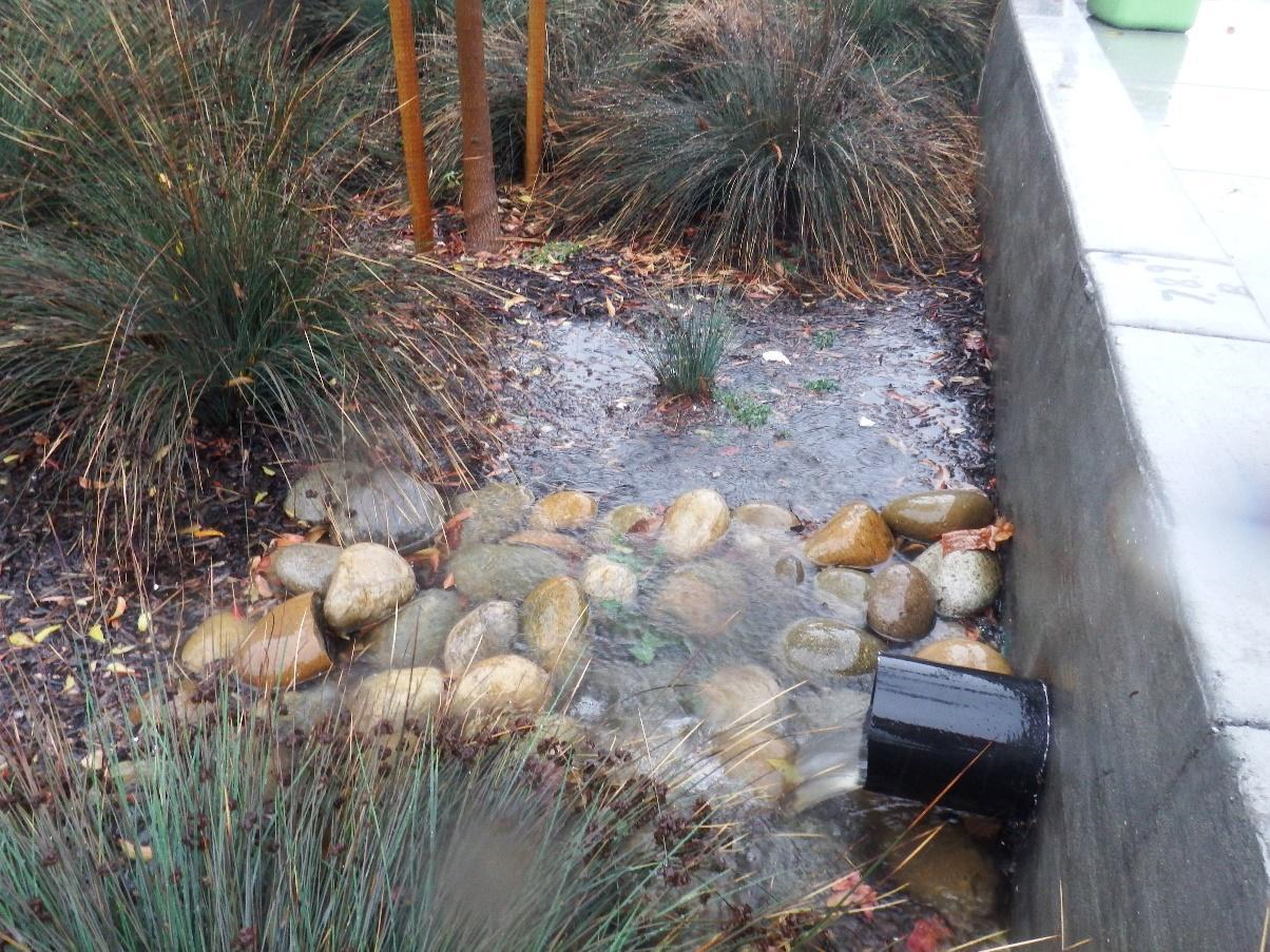
- Bioretention (with and without an underdrain as two different types) cells are small, vegetated, shallow depressions that serve to filter stormwater from impervious surfaces during rainfall events. Pollutants are removed from stormwater through adsorption, microbial activity, plant uptake, sedimentation, and filtration. Bioretention with out underdrains are more suitable to areas with higher soil filtration rates.
Figure 1. Bioretention unit on Osgood Road in Fremont, California (Source: Alicia Gilbreath)
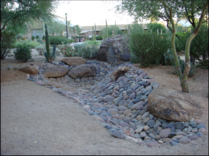
- Infiltration trenches are narrow trenches that have been back-filled with stone. Runoff is collected during storm events and stored in the void spaces of the gravel before being released back into the soil by infiltration.
Figure 2. Infiltration Trench (Source: GI Definitions and Details, J. Walker).
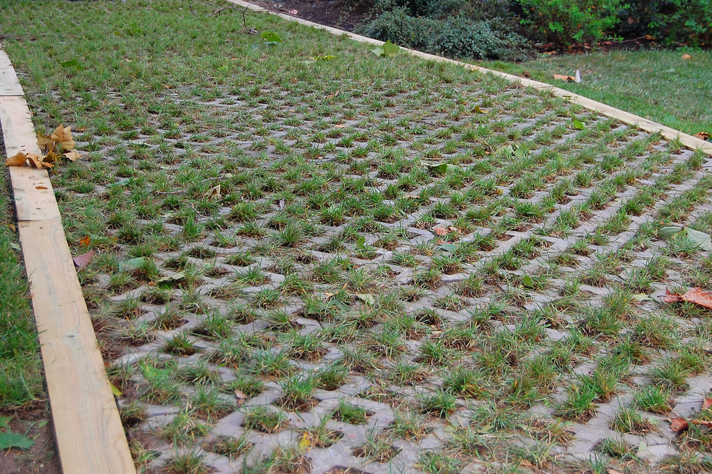
- Permeable pavement, or pervious pavement, is a porous surface laid over uniformly graded stones. It reduces runoff volume, peak discharge rates, pollutant loading, and runoff temperature.

Figure 3. Permeable pavement on Allston St., Berkeley, CA (Source: courtesy of Berkeleyside).
- Storm water wetlands collect runoff and store it in a permanent pool. Stormwater runoff drains into these wetlands and the plants and soils act as a filter for the stormwater.

Figure 4. Storm water wetlands (Source: GI Definitions and Details, J. Walker).
- Vegetated swales are broad, shallow channels with dense vegetation covering the sides of the slopes and bottom. They are designed to slow stormwater runoff and filter out particulate pollutants, and promote infiltration before reaching the stormwater drain.

Figure 5. Vegetated swale in Moss Beach, San Mateo County, California (Source: Nicole David)
- Wet ponds are used instead of a dry detention basin to provide flood control with enhanced amenities and aesthetics and improved pollutant removal. A wet pond provides similar benefits to stormwater wetlands, except they are typically deeper and may increase the temperature of runoff.

Figure 6. Wet pond (Source: GI Definitions and Details, J. Walker).
- Flow Through Planter boxes are bioretention systems with an impermeable lining. Water stored in the planter box is disharged through a pipe not through infiltration of native soils.
Figure 7. Flow Through Planter.
- Tree Well boxes are small-scale bioinfiltration systems that are highly adaptable for small places. Tree wells are designed to collect runoff to allowing excess water to infiltrate into native soil or be collected by an underdrain.

Figure 8. Tree well example by Filtera.
Site Locator Tool User Inputs
When using the Site Locator Tool, you have the option of using three (3) data input combinations (inputs are detailed below):

Regional Base Analysis
The regional base analysis component of the tool was developed by SFEI in 2011 via a grant received through the Critical Coastal Areas (CCA) program, and provides a map of suitable GI areas as a starting point for further analyses. This analysis has been more recently run to create regional suitability layers for the additional GI types. The regional base analysis output is provided in the GreenPlan-IT Site Locator Tool (in the file geodatabase base_analysis.gdb in the “data” folder).
For each GI feature type, identification of suitable locations in the regional base analysis was based on the following factors:
- Depth to water table
- Slope
- Hydrologic soil type
- Land use
- Liquefaction risk
- Surface imperviousness
Each factor was binned into groups that represented more or less suitable conditions for each GI type. These rankings were then weighted and used in a Categorical Weighted Overlay to identify locations that were suitable for each GI type.
Users may incorporate the base analysis provided either as an initial screening of suitable areas or during the ranking procedures (described below) but there are pros and cons. For example, incorporating the base analysis in the initial screening process provides a more refined (but exclusive) output since only locations that were deemed to be most suitable by the base analysis are included. Incorporating the base analysis in the ranking process provides a final output that is more inclusive of potential GI locations, and the results will not be limited to locations deemed suitable by the base analysis; rather, locations within the base analysis will receive a higher ranking than those not specified in the base analysis. This may be more desirable as many of the factors that were used to create the base analysis layer can be addressed by engineering and or design. That is, locations outside of the base analysis may still be possible locations for GI, however they may be more costly to install in those locations due to additional engineering and installation requirements (terracing due to slope, underdrain due to non-ideal soil type etc.). A city or county interested in saving costs by installing regionally applicable standard GI designs may need to take these issues into account when running the tool.
Refining Analyses
Municipalities may choose to adopt the base analysis as the sole input to their planning documents (not recommended in most circumstances) or to develop a refined analysis using additional regional datasets (provided with the GreenPlan-IT Site Locator Tool) and/or their own compilation of local city datasets. As with any simple model of a complex landscape, the scale and accuracy of input data will largely determine the scale and accuracy of the interpretative outputs. Therefore, when local higher quality data are available, we recommend these be incorporated. There are four (4) modules that may be used to facilitate a more refined analysis using available local data to improve the scale and accuracy (and relevance) of the tool outputs. These are:
- Locations Analysis
- Ownership Analysis
- Local Opportunities and Constraints Analysis
- Knockout Analysis
These modules are described in the following table and address weaknesses that would ensue if just the regional base analysis were to be used for planning feasible LID locations.

Regional Datasets
Regional datasets (in the file geodatabase RegionalDatasets.gdb in the “data” folder) are a collection of publicly available and SFEI-generated datasets that may be used in the Location, Ownership, Opportunities and Constraints, and/or Knockout Analysis modules.
See here for a description of the regional datasets provided.
Local Datasets
If municipality-specific data are available, users may choose to include these data in the Location, Ownership, Opportunities and Constraints, and/or Knockout Analysis modules.
See Tool Preparation, I. Compiling Local Datasets.
Introduction to File Structure and Necessary File Types
- Download the SiteLocatorTool_GreenPlanIT_SFEI.zip here.
- Navigate to the SiteLocatorTool_GreenPlanIT_SFEI.zip; right-click on the zip file→Extract All…→Extract the contents to a folder.
- If you would like to store the tool elsewhere, move the extracted folder and its contents to your desired location.
SFEI has provided the GreenPlan-IT Site Locator tool (with ancillary files), the regional base analysis, and the regional datasets in a preset folder schema, as shown below. If using local datasets, the user should reference the folder schema to determine the locations and formats of any compiled data. This will be described in detail in Tool Preparations.

Tool Preparations
If you will not be using regional datasets (provided) or local datasets, skip to Run Tool: 1 – Site Locator Tool.
If you will not be using local datasets, skip to Tool Preparations, Preparing Analysis Tables.
If you will be using local datasets, continue with the next step which is compiling data sets.
Compiling Datasets
- Create a new file geodatabase for your local datasets in the “data” folder.
- We recommend renaming your file geodatabase using the convention YourMunicipalityNameDatasets.gdb (i.e. ContraCostaDatasets.gdb).
- Save/export any relevant datasets to this new file geodatabase.
- The default spatial reference used by the GreenPlan-IT Site Locator Tool is NAD 1983 California Teale Albers (EPSG: 3310). As a best practice, we recommend projecting any local datasets to this spatial reference; however, this is not a requirement.
Preparing Analysis Tables
When preparing to run the GreenPlan-IT Site Locator Tool, the user will be required to specify if any additional refined analyses (Location, Ownership, Opportunities and Constraints, and/or Knockout Analysis) will be used. The user may select any combination of refined analyses when running the GreenPlan-IT Site Locator Tool (i.e. any combination of 0 - 4 analyses).
If using any of these additional refined analyses (Location, Ownership, Opportunities and Constraints, and/or Knockout Analysis), the user will be required to provide an accompanying table (templates provided by SFEI in the “tables” folder) for each analysis type desired. Each table provides details of the regional/local dataset(s) being used in the specified analysis. For each analysis type selected, the user will determine which regional/local datasets should be included.
If including Location Analysis
- Open locations.csv in the “tables” folder.
- For each regional/local dataset to be included, use the locations.csv, Field Metadata to determine entries in each table field. An example of a completed locations.csv table is here: Example locations.csv.
- Save locations.csv.
If including Ownership Analysis
- Open ownership.csv in the “tables” folder.
- For each regional/local dataset to be included, use the ownership.csv, Field Metadata to determine entries in each table field. An example of a completed locations.csv table is here: Example ownership.csv.
- Save ownership.csv.
If including Opportunities and Constraints Analysis
- Open opportunities_and_constraints.csv in the “tables” folder.
- For each regional/local dataset to be included, use the opportunities_and_constraints.csv, Field Metadata to determine entries in each table field. An opportunities_and_constraints.csv table is here: Example opportunities_and_constraints.csv.
- Ranking process:
- To fill out the opportunities and constraints table, first you list all of the layers under layer name with it’s associated layer path, alias, query, and buffer size.
- Then you rank that layer as either a positive or negative factor for ranking a GI location. If it is negative, type “-1” under “rank” if positive then type “1”.
-
Next, you organize all layers into factors such as:local development considerationinstallation feasibilitycommunity needsfunding opportunitieswater quality, etc.(you can also make up your own factors and/or put all layers within one or two factors).
- Factor weight: Assign a weight to each factor such that the sum of all factor weights = 1 (for example, .25 for Local Development and .75 for installation feasibility if those were the only two factors you were using). A higher number indicates a higher weight for a particular factor. Provide this value to each layer row that the factor applies to.
- Layer weight: Within each factor, assign a weight to each layer so that the sum of the layer weights within each factor = 1. A higher number indicates a higher weight for a particular layer. If there is only one factor within that layer then the weight of that layer as 1.
- This table then runs nested weighted sums in order to produce a final ranking for each lid potential location. Note, you may choose to edit the opportunities and constraints table after viewing results. This is often an iterative process in order to create the most useful output for a user. Or you could purposely run it different ways for each neighborhood if there are specific local interests that are more or less important.
- Save ownership.csv.
If including Knockouts Analysis
- Open knockouts.csv in the “tables” folder.
- For each regional/local dataset to be included, use the knockouts.csv, Field Metadata table to determine entries in each table field. An example of a completed knockouts.csv table is here: Example knockouts.csv.
- Save knockouts.csv.
Preparing GI Size Table
SFEI has also provided lid_size.csv, which lists each GI type along with a suggested average area (square feet). When running the Site Locator Tool, the GI Size Table is used to remove GI locations that do not meet the minimum area specified. This table is also required if the user plans on running the Optimization Precursor Tool to generate inputs for the GreenPlan-IT Optimization Tool.
Use of the gi_size.csv table is optional, but recommended.
If including the GI Size Table…
- Open gi_size.csv in the “tables” folder.
- Adjust the values in the “ave_size_sqft” as desired/necessary. An example of a completed lid_size.csv table is here: Example gi_size.csv. See gi_size.csv, Field Metadata for field descriptions.
- Save gi_size.csv.
Loading the GreenPlan-IT Toolbox
- Open a new map document in ArcMap.
- If the ArcToolbox Window is not open, click the ArcToolbox button
 on the Standard Toolbar.
 - If the GreenPlan-IT Tool is not visible in the ArcToolbox Window…
- Right-click ArcToolbox.
- Select Add Toolbox…

- Browse to the location of the SiteLocatorTool_GreenPlanIT_SFEI folder, and select the GreenPlan-IT.pyt toolbox file.

- Click Open.
- The GreenPlan-IT Toolbox has now been added to the ArcToolbox Window.

1 - Site Locator Tool
The Site Locator Tool is the primary tool in GreenPlan-IT Toolbox. This tool identifies (and ranks, when Opportunities and Constraints Analysis is used) feasible locations for GI development.
Hardware/ ESRI Software Requirements
- 8 GB RAM (required); 16 GB RAM (recommended)
- 64-bit background geoprocessing
- Spatial Analyst Extension
Running the Tool
- Double-click 1 – Site Locator Tool in the GreenPlan-IT Toolbox.
- The tool will open to the following interface:

- Output Directory: Select the folder where you would like the site locator tool outputs to save. We recommend that the character length of the output directory be < 100 characters.
- Set the extent: You may set the extent by (a) selecting an Area of Interest or (b) setting a Custom Area of Interest using a polygon feature class with a single feature containing the desired boundary area.
- To select an Area of Interest: Use the Area of Interest dropdown menu and select the desired area.

- To select a Custom Area of Interest: Select "[Custom Area of Interest]" under the "Area of Interest" field. This activates the "Custom Area of Interest (optional)" field which you can then specify the polygon feature class containing your custom boundary.
- To select an Area of Interest: Use the Area of Interest dropdown menu and select the desired area.
- GI Types: Select at least one GI type to include in the Site Locator analysis.
- Modules (optional): Select the modules/additional analyses to be included when running the tool.
- Restrict Output to Base Analysis Extent: SFEI has provided a base analysis for each of the nine (9) GI types. Check to restrict the final outputs to only areas that overlap the regional suitability layer for each GI type.
- Note: The base analysis layers can be incorporated two ways: (1) Check “Restrict Output to Base Analysis Extent”to exclude all locations that are NOT identified as suitable area for each GI type in the base analysis. (2) Do not check “Restrict Output to Base Analysis Extent” to prevent results from being limited to locations identified as suitable for each GI type in the base analysis. You may still include the base analysis layer in the Opportunities and Constraints module and run the tool for that type of GI only, in order to rank locations that fall within the base analysis areas as higher. This second option may be the preferable method. See Preparing Analysis Tables.
- Module Tables (optional): Table paths should only be provided for selected modules/analyses.
- Locations Table: If you selected the Location Analysis module, navigate to and select your locations.csv table.
- Opportunities and Constraints Table (Default and GI specific): If you selected the Opportunities and Constraints Analysis module, navigate to and select your opportunities_and_constraints.csv table for each GI type.
- Note: you can specify a "Default" Opportunities and Constraints Table which will be used for any GI types that do not have a GI specific Opportunities and Constraints Table specified.
- Ownership Table: If you selected the Ownership Analysis module, navigate to and select your ownership.csv table.
- Knockout Table: If you selected the Knockout Analysis module, navigate to and select your knockouts.csv table.
- GI Size Table: If using average GI sizes in the Site Locator analysis, navigate to and select your gi_size.csv table.
- Export KMZ of Outputs: Check to generate KMZs of the GI locations; these may be viewed in Google Earth or Google Maps.
- Note: The KMZs generated by the GreenPlan-IT Site Locator Tool contain simplified feature polygons and should be used for general viewing purposes only. Any analysis should be performed using the feature classes in the file geodatabase.
- Save PNG of Outputs: Check to export a PNG map of the outputs. The legend provided with the tool will have to be added manually.
- Save PDF of Outputs: Check to export a PDF map of the outputs. The legend provided with the tool will have to be added manually.
- Click OK to run. (The tool may take several hours to run to completion, depending on the size of the area of interest, the number of GI types selected, and the number of modules included.)
Understanding the Outputs
Final File Geodatabase of Outputs
As the GreenPlan-IT Site Locator Tool runs, feature classes and table outputs will be saved in a file geodatabase in the Output Directory. Many of these are projected copies of the input data or intermediate analyses; however, the final GI locations for each selected GI Type will be saved in the following format:

Notes:
- A ranking will only be applied when the Opportunities and Constraints Analysis has been applied.
- Feature classes ending in “_private” or “_public” separate GI locations into the private and public domains, respectively. These feature classes are only generated if a distinction between private/public areas has been made in the Location Table and/or Ownership Table.
GI Location Feature Class Description
Each final GI location feature class will follow this field schema: Feature Class Metadata.
GI Area by Rank
For each GI type selected, the Site Locator Tool will generate a summary of GI areas (acres) by 0.1 rank intervals. These tables will have names according to the format, “GI_Area_by_Rank_GI Type_yyyy.mm.dd.csv”.
Unranked areas will be assigned rank = 9999.
KMZ Exports
If Export KMZ of Outputs was selected, a “KMZ_OUT_yyyy.mm.dd_hh.mm.ss” folder will be saved in the Output Directory. Each KMZ represents a geographic quadrant of the area of interest. A set of KMZ quadrants is made for each selected GI type (one set each for all locations, and private locations and public locations, where applicable).
For example, the KMZ exports for the Bioretention GI Type with Ownership Analysis (i.e. private/public distinction) and Opportunities and Constraints Analysis (i.e. ranked) would look like this:

Additionally, if ranked, LID location polygons are symbolized according to the following color scheme:

Unranked areas will be assigned rank = 9999.
Messages and Summaries
The GreenPlan-IT Tool auto-generates a message and summary file each time the Site Locator Tool is run:
GI_Site_Suitability_AreaOfInterest_yyyy.mm.dd_hh.mm.ss_messages.txt – this is a text record of input tool parameters and execution messages/errors.
GI_Site_Suitability_AreaOfInterest_yyyy.mm.dd_hh.mm.ss_summary.csv – this is a record of input tool parameters and completion times for any module analyses, as well as the total tool completion time.
2 – Optimization Precursor Tool
The Optimization Precursor Tool generates the required inputs for the GreenPlan-IT Optimization Tool. This tool calculates the total area of each GI type within each sub-basin (produced during hydrologic modeling of the area). Additionally, the Optimization Precursor Tool calculates the number of possible GI locations within each sub-basin based on the minimum GI areas defined in the GI Size Table.
Note: Where multiple GI locations overlap, the overlap area is divided amongst the relevant GI types. In this way, total area is conserved.
Running the Tool
- Double-click 2 – Optimization Precursor Tool in the GreenPlan-IT Tools toolbox.
- The tool will open to the following interface:

- Input Geodatabase: Select the file geodatabase generated from the Site Locator Tool. The name of this geodatabase will have a name similar to LID_Site_Suitability_AreaOfInterest_yyyy.mm.dd_hh.mm.ss.gdb.
- Output Directory: Select the folder where you would like the Optimization Precursor Tool outputs to save.
- Sub-basin Feature Class: Select a polygon feature class containing the sub-basin boundaries for the area of interest.
- Sub-basin ID: Use the dropdown menu to select a unique ID field from the Sub-basin Feature Class. If a unique ID field does not exist, use the Object ID field.
- GI Types: Select the GI types to include in the Site Locator analy.
- GI Size Table: Navigate to and select your lid_size.csv table.
- GI Size Table Unit: Select the unit of measure in the GI size table: (SQUARE) FEET or (SQUARE) METERS.
- Ownership Domains: Use the dropdown menu to select the ownership domain.

- Click OK to run.
Understanding the Outputs
The primary output of the Optimization Precursor Tool is the table “Sub-basin_Model_Input_yyyy.mm.dd_hh.mm.ss.csv”. This table summarizes the total area by GI type in each sub-basin; it also estimates the number of potential GI installations (by type) in each sub-basin, based on the total area and average GI sizes as specified in the GI Size Table.
Note: Where multiple GI locations overlap, the overlap area is divided amongst the relevant GI types. In this way, total area is conserved.
The specific fields/field names included in this table will vary based on the user inputs.
Modeling Tool
GreenPlan Modeling Tool User Guidance
Prepared by
SAN FRANCISCO ESTUARY INSTITUTE
4911 Central Avenue, Richmond, CA 94804
Phone: 510-746-7334 (SFEI)
Fax: 510-746-7300
Table of Contents
1. INTRODUCTION……..……………………………………………………………………...................1
2. DOWNLOAD AND SET UP SWMM. ……………………………………………………..............1
3. MODEL DEVELOPMENT………………………………………………………………….................2
3.1 Input data ..................................................................................................2
3.2 Watershed Delineation................................................................................3
3.3 Hydrology Calibration.................................................................................3
3.4 Water Quality Calibration............................................................................5
3.5 GI Simulation..............................................................................................6
4. MODEL LIMITATIONS……………………..……………………………………………...................6
5.REFERENCES....................................................................................................7
1. INTRODUCTION
The modeling tool of the GreenPlan-IT toolkit is a spatially distributed hydrologic and water quality model that simulates runoff quantity and quality from primarily urban areas as well as hydrologic performance of Green Infrastructure (GI). The tool is built upon the publicly available EPA Storm Water Management Model (SWMM) (Rossman, 2010), a dynamic rainfall-runoff simulation model used for single event or long-term (continuous) simulation of runoff quantity and quality and is used for planning, analysis and design related to stormwater runoff management, combined and sanitary sewers, and other drainage systems in urban areas. Within the toolkit, this tool is used to establish the baseline hydrology and water quality conditions through the characterization of the modeled watershed before any new management activities are implemented; identify high-yield runoff and pollution areas; and evaluate relative effectiveness of implementing GIs across different areas within a watershed, based on their potential for reducing runoff volume or contaminant loads.
The modeling tool currently utilizes three modules of SWMM: (1) the hydrological module; (2) the pollutant module; and (3) the GI module. The hydrologic and pollutant modules are used to simulate the generation, transport, and fate of stormwater runoff and associated pollutants from the landscape. The GI module utilizes stormwater runoff from the hydrologic module as the forcing function for GI simulation to estimate any reduction made from GI implementation by performing without and then with the GI scenarios simulation.
Since SWMM is an established public domain model, users of GreenPlan-IT can obtain existing SWMM documentation from the EPA SWMM website (briefly discussed in next section) for guidance on how to set up and run the model. As such, this manual will not provide a detailed description of SWMM, its strengths and weaknesses, or software and hardware requirements, nor step by step instructions on model setup as a regular user manual would do. Rather, it will focus on providing guidance on model development and application. Before running GreenPlan-IT, users should familiarize themselves with the SWMM user guidance.
The Green Plan-IT modeling tool is intended for knowledgeable users familiar with technical aspects of watershed modeling more generally and SWMM ideally.
2. DOWNLOAD AND SET UP SWMM
The SWMM installation program, user’s manual, as well as source code are available at the EPA SWMM website: http://www2.epa.gov/water-research/storm-water-management-model-swmm.
Users can follow the instructions provided at this link to download and install SWMM on a PC. In particular, users will need to download:
- Self-extracting installation program for SWMM5.0. Run this .exe file will install SWMM on a PC. The detailed instruction on model installation and pertinent software/hardware requirements are provided in the SWMM user manual.
- SWMM5.0 User’s Manual. This is the main SWMM document that provides step-by-step instructions on how to set up and get started with SWMM, as well as detailed description on SWMM structure and various functionalities and options (graphical user interface, the project files, and how to build a network model of a drainage system, use the study area map, run a simulation, and the various ways to view model results).
In addition, users are strongly encouraged to download and go through the ‘SWMM Applications Manual’ to help expedite their use of SWMM. It contains nine worked-out examples that illustrate how to use SWMM to model some of the most common types of stormwater management and design problems. In some cases, advanced users may also want to download and manipulate the SWMM source code to meet their specific needs.
3. MODEL DEVELOPMENT
The model development for a SWMM application is similar to most watershed modeling projects and usually begins with collecting and reviewing input data, followed by setting up the model, and calibrating the model to match local data. Once the model development is completed, the model can then be used to answer management questions by simulating various management scenarios. In the case of this project, the developed modeling tool is used to drive GI simulation.
3.1 Input Data
The development of a hydrologic model requires all water sources and sinks to be included in the model. The data collection process involves a thorough compilation and review of information available for the study area. It generally includes gathering applicable regional and site-scale GIS data layers, digital elevation model (DEM) data, stream networks, soil, land use, critical source information, and monitoring data for calibration and validation. A summary of typical data needs for SWMM development is provided in Table 3-1.

3.2 Watershed Delineation
Watershed delineation is a process that divides a watershed into smaller sub-basins to analyze watershed behavior. Consistent with the lumped nature of the model, each sub-basin is modeled as a homogeneous unit with spatially averaged descriptive properties. Watershed delineation is normally done by GIS analysis using topographical data. The watershed delineation will establish a representation of the study area, and ideally, locally derived higher-resolution site scale data should be used. The proper spatial scale of a modeling project is usually determined through professional judgment and needs to take into account important factors such as the project goals, size of the study area, spatial scale of crucial input data, and model run time. For a stormwater management project, watershed delineation should strike a balance between a meaningful size of sub-basins for guiding GI implementation and demand on computer run time.
3.3 Hydrology Calibration
Similar to other modeling efforts, a critical first step for SWMM development is to calibrate the model using local data, before it is used by municipalities to simulate GI scenarios for their local watersheds. A hydrologic calibration is typically done by means of an iterative process of trial and error, by adjusting the parameters within the established range until modeled flow rates match the timing, magnitude, and total volume of the field-observed streamflow data. The model calibration is necessary to ensure that a representative baseline condition is established with a high degree of confidence in its applicability to form the basis for comparative assessment of various management scenarios.
SWMM is associated with a large number of spatially variable parameters that describe the characteristics of individual sub-basins. A subset of the model parameters associated with frequent storm events (impervious percentage, subcatchment width, Manning’s roughness, depression storage, and soil infiltration parameters) are most sensitive and typically used as hydrologic calibration parameters. A brief discussion of each parameter follows.
- Imperviousness
The percentage of impervious area is often the most sensitive parameter, strongly influencing both total runoff volume and peak flows. The initial estimate of imperviousness is usually determined by GIS analysis of land use/land cover data. During calibration, the percent¬age of imperviousness is adjusted up/ down as necessary to be consistent with known conditions in the study area and to obtain a good adjustment of the hydrograph.
- Subcatchment width
The subcatchment width is computed by dividing the subcatchment area by the travel length. This is an abstract basin parameter and is commonly used as a “tuning parameter” for model calibration because of the uncertainty associated with determining the travel length of stormwater runoff. Increasing the travel length decreases the subcatchment width which creates a more attenuated response to storm events.
- Manning’s (surface) roughness
Manning’s roughness coefficient is used in SWMM for the routing of overland flows and has an influence on the timing of peak flows. Separate roughness coefficients are applied to pervious versus impervious surfaces. Typical values are as follows:
- Impervious: 0.015 (dimensionless)
- Pervious: 0.250 (dimensionless) or higher in heavily vegetated areas
Manning’s n values are often assigned a default value (from typical value suggested in SWMM User Manual, GIS analysis of land cover type and/or literature review), and then adjusted within the range of the established values in the literature to ensure they are representative of current basin conditions.
- Depression storage
Depression storage refers to the storage depth associated with surface depressions that are filled prior to runoff. The potential depression storage is related to the surface roughness coefficient; thus, separate values are required for pervious and impervious surfaces. Typical values are as follows:
- Impervious: 0.1 inch
- Pervious: 0.2 inch
Depression storage affects sensitivity of runoff to precipitation and is negatively and weakly correlated to surface runoff. Adjusting this parameter could improve model performance, but the improvement is often limited.
- Soil infiltration parameters
SWMM offers three choices for modeling infiltration: the Horton's Equation, the Green-Ampt Method, and the Curve Number Method, each requiring a different set of input parameters. Regardless of the method used, the infiltration parameters are closely correlated to hydrologic characteristics of the soil groups. Regional data available from the NRCS in the State Soil Geographic Database (STATSGO) is commonly used in lieu of local soil information to determine the default values and allowable ranges for each parameter. The calibration process then involves varying the parameters within their defined bounds in an effort to optimize the model.
Other less sensitive parameters required by SWMM such as subcatchment slope and percent of impervious area with no depression storage can be assigned a default value based on recommendation from the SWMM User Manual, GIS analysis and/or literature review.
3.4 Water Quality Calibration
SWMM can simulate the production of pollutant concentrations and loads associated with stormwater runoff. The model is capable of analyzing the buildup, washoff, transport and treatment of a variety of water quality constituents such as sediment, heavy metals, and nutrient. Because the SWMM uses the buildup-washoff formulation that assumes urban runoff quality constituents behaving in some manner similar to “sediment” of sediment transport theory, it works well for constituents that are transported in solid form, either as particulates or by adsorption onto soil particles, but not for constituents that are transported primarily in a dissolved state, e.g., NO3. Water quality parameters are defined for buildup and washoff of each pollutant and include maximum surface build-up, surface build-up rate and wash-off coefficients. These parameters are land use specific and are primary parameters used for water quality calibration.
The water quality calibration is also made by means of an iterative process of trial and error, by adjusting the parameters within the established range, and comparing (numerically and graphically) the modeled results (usually pollutant concentrations) with the measured data, until a good fit is obtained. The water quality calibration has often proved more difficult than the hydrology calibration, due largely to the lack of high resolution calibration data, both temporally and spatially. Therefore, the calibration procedure should also incorporate the comparison of the outcomes with a reasonable conceptual understanding of the likely variation of pollutant sources, erosion, and transport processes in the landscape that is water quality parameter specific. The outcome of the water quality simulation should at least compare closely with this conceptual model and follow the reasonable likelihood that pollutant production should vary more between each sub-basin than flow production. For example, flow production between sub-basins normally varies by 2-4-fold between the least to the most imperious sub-basins whereas it is not uncommon for pollutant loads to vary by any magnitude between sub-basins by 5-100-fold.
3.5 GI Simulation
SWMM can simulate the hydrologic performance of seven GI types: Permeable Pavement, Rain gardens, Green roofs, Street planters, Rain barrels, Infiltration trenches, and Vegetative swales (Rossman, 2010). The GI simulation is usually performed after SWMM is developed for a watershed using local data, to quantify any runoff reduction associated with GI implementation.
For SWMM to simulate a GI, users need to specify GI design, location, and treatment area within a watershed. The types of GI compartments are: storage, underdrain, surface, pavement and soil. GI controls are represented by a combination of these vertical layers whose properties are defined on a per-unit-area basis. These compartments are GI specific and the SWMM5 user manual (Rossman, 2010) provides a detailed description on the configuration of each GI type.
4. MODEL LIMITATIONS
Despite its capacities for addressing many stormwater problems, SWMM has a number of limitations that users need to be cognizant of before using the model.
- Although it has been widely used elsewhere, the model is not directly applicable to large-scale, non-urban watersheds, and performs best in urbanized areas with mainly impervious cover within drainage area of interest.
- The model is not applicable to forested areas or irrigated cropland because of lack of parameterization for evapotranspiration in the model.
- Water quality simulations follows a simple buildup-washoff process, as such, the model is best suitable for modeling pollutants in particle form or closely associated with sediment, and less applicable to pollutants in dissolved forms (i.e. nitrogen species).
- The model only computes sediment delivery from overland flow. The model does not contain mechanisms for sediment deposition and transport within a river channel.
- The model is currently only capable of simulating hydrologic performance of selected GI types. The mechanistic simulation of pollution reduction is not built into the model. Additional programing by the user is required for simulating load reduction within the GI types.
5. REFERENCES
Rossman, L. A (2010). Storm Water Management Model User’s Manual, Version 5.0, U.S. Environmental Protection Agency. Office of Research and Development. EPA/600/R-05/040.
USEPA (2011). Report on Enhanced Framework (SUSTAIN) and Field Applications for Placement of BMPs in Urban Watersheds, EPA 600/R-11/144. U.S. Environmental Protection Agency, Office of Research and Development, Cincinnati, OH.
Optimization Tool
![]() Optimization Tool User Manual 2020.pdf
Optimization Tool User Manual 2020.pdf
Optimization Tool User Manual
Prepared by
SAN FRANCISCO ESTUARY INSTITUTE
4911 Central Avenue, Richmond, CA 94804
Phone: 510-746-7334 (SFEI)
Fax: 510-746-7300
July 2020
Table of Contents
1. OVERVIEW
1.1 GreenPlan-IT
1.2 Optimization Tool Overview
1.3 Optimization Algorithm
1.4 Structure of Optimization Tool
2. FORMULATION OF OPTIMIZATION
3. INSTALL OPTIMIZATION TOOL
4. RUN OPTIMIZATION TOOL
4.1 Create Input Files
4.2 Run the Tool
5. REVIEW AND INTEPERATE OUTPUTS
6. FUTURE UPGRADES
7. REFERENCES
OVERVIEW
1.1 GreenPlan-IT
GreenPlan-IT is a planning tool that was developed over the past five years with strong Bay Area stakeholder consultation. GreenPlan-IT was designed to support the cost-effective selection and placement of Green Infrastructure (GI) in urban watersheds through a combination of GIS analysis, watershed modeling and optimization techniques. GreenPlan-IT comprises four distinct tools: (a) a GIS-based Site Locator Tool (SLT) that combines the physical properties of different GI types with local and regional GIS information to identify and rank potential GI locations; (b) a Modeling Tool that is built on the US Environmental Protection Agency’s SWMM5 (Rossman, 2010) to establish baseline conditions and quantify anticipated runoff and pollutant load reductions from GI sites; (c) an Optimization Tool that uses a cost-benefit analysis to identify the best combinations of GI types and number of sites within a study area for achieving flow and/or load reduction goals; and (d) a tracker tool that tracks GI implementation and reports the cumulative programmatic outcomes for regulatory compliance and other communication needs. The GreenPlan-IT package, consisting of the software, companion user manuals, and demonstration report, is available on the GreenPlan-IT web site hosted by SFEI (http://greenplanit.sfei.org/).
1.2 Optimization Tool Overview
The optimization tool of GreenPlan-IT can be used to identify and prioritize the most cost-effective GI implementation among the many options available in urban and developing areas. The tool uses an evolutionary optimization technique, Non-dominated Sorting Genetic Algorithm II (NSGA-II), to systematically evaluate the benefits (runoff and pollutant load reductions) and costs associated with various GI implementation scenarios (location, number, type, and size of GI) and identify the most cost-effective options for achieving desired flow mitigation and pollutant reduction at minimum cost. Figure 1-1 shows an example GI scenario that specifies types and numbers of GI features within different sub-basins (locations). Within GreenPlan-IT, the optimization tool is structurally designed as a standalone module to provide flexibility for the user community, but it needs interaction with other tool components to function. The optimization tool uses the site information generated from the GIS Site Locator tool as input data and interacts with the modeling tool during the search process in an iterative and evolutionary fashion to generate viable GI scenarios and compare their performance. Therefore, running the tool requires the running of both the Site Locator Tool and Modeling Tool (http://greenplanit.sfei.org/).
The optimization tool is designed to help local watershed planning agencies to develop stormwater management plans and coordinate watershed-scale investments to meet their program needs. It is intended for knowledgeable users familiar with the physics of GI and the technical aspects of watershed modeling. The tool outputs, combined with other site specific information.
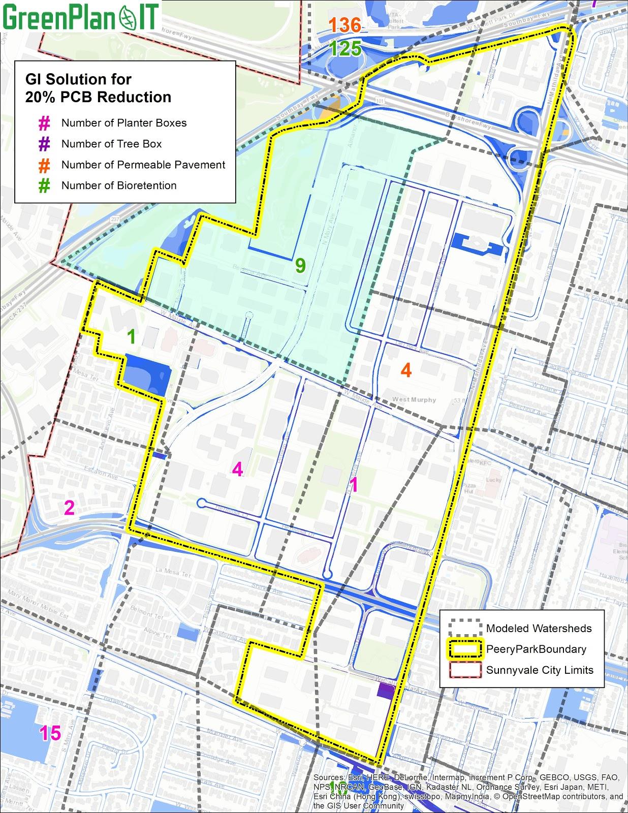
Figure 1-1. Example GI scenario showing types and numbers of GI features (color coded, see map legend) within different sub-basins (locations)and management requirements, can be used to develop watershed-scale Green Infrastructure master plans.
1.3 Optimization Algorithm
Belonging to the family of evolutionary optimization techniques, NSGA-II is one of the most efficient and widely used multi-objective optimization algorithms that is capable of producing optimal or near-optimal solutions that describe tradeoffs among competing objectives (Deb, et al, 2002). NSGA-II incorporates a non-dominating sorting approach that makes it faster than any other multi-objective algorithm and uses a crowded comparison operator to maintain diversity along the Pareto optimal front (Srinivas and Deb, 1994). Examples of the use of NSGA-II for addressing environmental problems have been reported in the EPA SUSTAIN applications (USEPA 2009) as well as many case studies in the literature (Bekele and Nicklow, 2007; Bekele, et al, 2011; Maringanti, et al, 2008; Rodriguez, et al, 2011). The major operation steps of NSGA-II are described below.
-
Creation of First Generation
The algorithm begins with random generation of an initial population of potential solutions. The population is sorted based on the concept of Pareto dominance (non-domination) into each front. A solution is non-dominant to another solution when itperforms no worse than the other solution in all objectives, and better than the other solution in at least one objective. At the end of the sorting, each solution is assigned a fitness (or rank) equal to its non-dominant level, with a smaller rank indicating that the solution is dominated by fewer other solutions. In addition, a crowding distance, defined as the size of the largest cuboid enclosing a solution without including any other solution in the population, is calculated for each individual solution as a measure to maintain solution diversity. Large average crowding distance results in better diversity in the population.
-
Optimization Process
In the first step of the optimization process, parent populations are selected from the population by using binary tournament selection based on the rank and crowding distance. An individual solution is selected if the rank is lesser than the other solutions or if crowding distance is greater than the other solutions. The selected population generates an offspring population of the same size from the processes of crossover and mutation. The combined population of the current parent and offspring is sorted again according to non-domination and only the best N individuals are selected to form a new parent population, where N is the population size. Elitism is ensured in this step because both the parent and the child populations are used in the sorting. Comparison of the current population with previously identified non-dominated solutions are performed at each iteration. The new parent population is then used to create a new child population, and the process continues until the stopping criteria are met. At that point, the optimization is considered converged at an optimal front and the process can be stopped.
-
Stop Criteria
The users can stop the NSGA-II using some user-defined stop criteria. The commonly used criteria include maximum number of iterations; no change in the new parent population for two consecutive loops; and no tangible improvement for the fitness function after a certain number of iterations.
1.4 Structure of Optimization Tool
Structurally, the optimization tool is built around three functionalities each supported by a group of subroutines: Optimizer, GI performance evaluator, and cost calculator. The optimizer serves as the optimization engine that generates GI scenarios and drives the search process through the NSGA-II algorithm. The GI performance evaluator is used to create input files for the modeling tool to incorporate the generated GI scenarios, runs the model with new input files, and passes GI performance data generated by the model back into the optimizer. The cost calculator is used to estimate the cost of each GI scenario and to pass that information into the optimizer.
The three function groups work hand-in-hand in an iterative and evolutionary fashion to search forthe best GI solutions that meet the user’s specific conditions and objectives. During the search process, new GI scenarios are generated through the optimizer within the search space defined by the universe of feasible locations that are identified by the GIS Site Locator tool, the GI performance for each of the scenarios are evaluated, and costs for each are estimated. The optimizer then systematically compares the cost and performance data and modifies the search path to generate a new set of viable GI options and repeats the process until the set criteria to end the iteration are reached. Figure 1-2 presents a conceptual overview of the tool.
The optimization tool was written in FORTRAN language. The coding of NSGA-II was verified with example problems provided at Deb, et al (2002) to make sure the optimization algorithm was implemented correctly. The maximum number of iterations was used as stop criteria.
2. FORMULATION OF OPTIMIZATION
The formulation of the multi-objective optimization problem involves defining optimization objectives, determining decision variables, and identifying associated constraints.
-
Optimization Objectives
The optimization objectives used in this tool are to: 1) minimize the total relative cost of GI scenarios; and 2) maximize the total PCBs load reduction within a study area.
-
GI Types and Design Specifications
Four GI types - bioretention, permeable pavement, tree well (proprietary media), and flow-through planter, are currently included in the Optimization Tool, but other types could be added by an advanced user. Each GI type is assigned typical size and design configurations that were reviewed and approved by the Technical Advisory Committee (TAC) (Table 2-1). These design specifications remain unchanged during the optimization process. But if a user wants to use different design specifications for these four types, or have four totally different GI types to fit their specific needs, this can be easily achieved by changing the GI attributes in both the SWMM template file and the LID input file for optimization (discussed in Section 3).
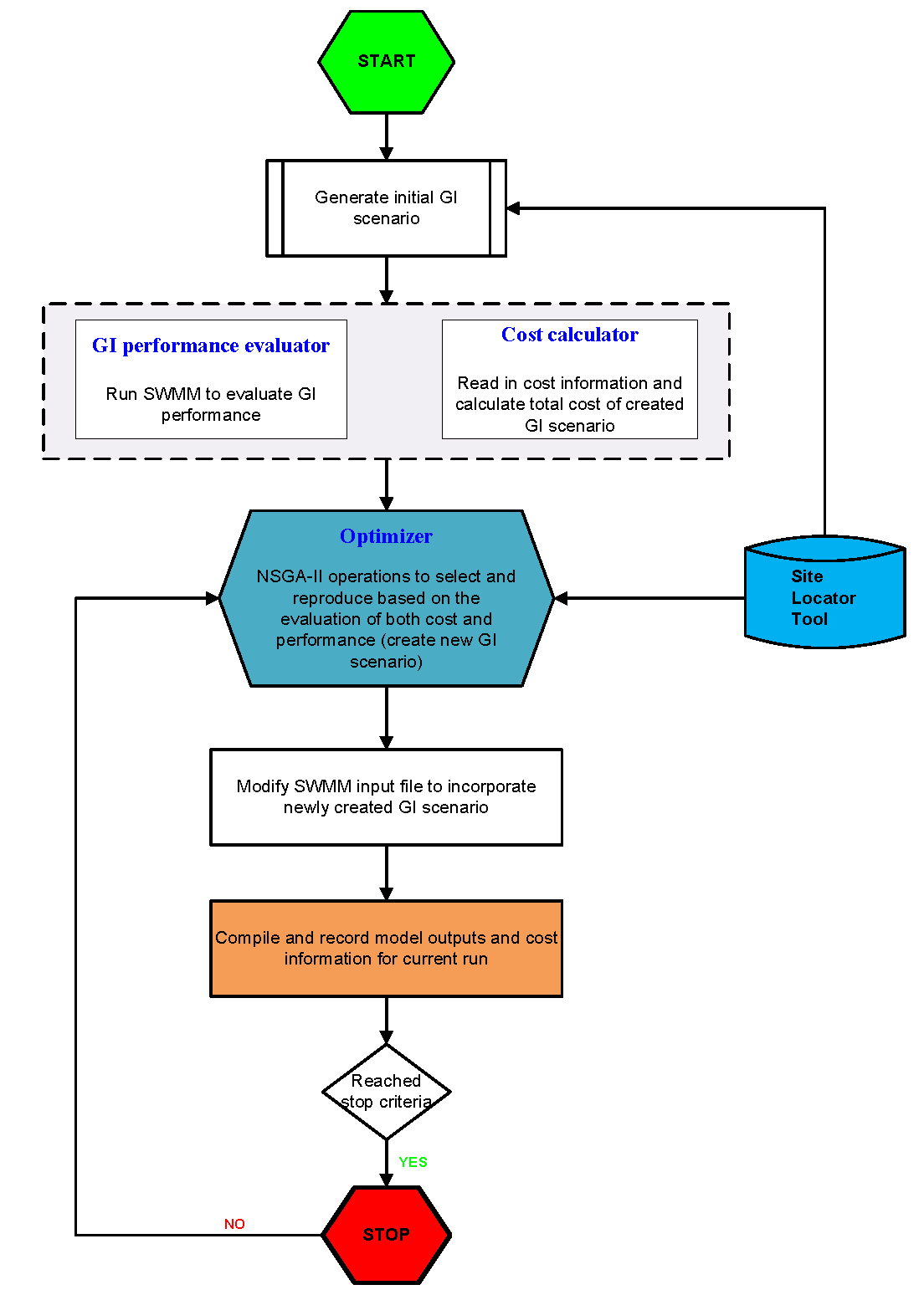
Figure 1-2. Flowchart of Optimization Tool
While current template files for the tool only include four GI types, the tool is set up to take up to six GI types. If a user is interested in other GI types, they can specify them in both the SWMM file and optimization input file, but including more than six GI types will require minor changes and recompilation of source code.
Table 2-1. GI types and configurations currently used in the Optimization Tool.
|
GI Specification |
Surface area (sf) |
Surface depth (in) |
Soil media depth (in) |
Storage depth (in) |
Infiltration rate (in/hr) |
Underdrain |
Sizing factor* |
Area treated (ac) |
|
Bioretention |
500 (25x20) |
9 |
18 |
12 |
5 |
Yes: Underdrain at drainage layer |
4% |
0.29 |
|
Permeable pavement |
5000 (100x50) |
0 |
24 |
100 |
Yes: 8 inch for underdrain |
50% |
0.23 |
|
|
Tree well |
60 (10x6) |
12 |
21 |
6 |
50 |
Yes: Underdrain at bottom |
0.4% |
0.34 |
|
Flow-through planter |
300 (60x5) |
9 |
18 |
12 |
5 |
Yes: Underdrain at bottom |
4% |
0.17 |
* In relation to the drainage management area of the unit.
-
Decision Variables
In the optimization, since GI design specifications were user specified and remained constant, the decision variables were therefore the number of units of each of the GI types in each of the subbasins within a study area. For each applicable GI type, the decision variable values range from zero to a maximum number of potential sites as specified by the boundary conditions identified by the GIS SLT.
-
Constraints on GI Locations
For each GI type, the number of possible sites is constrained by the maximum number of potential sites identified by the GIS locator tool. The decision variables were also constrained by the total area that can be treated by GI within each subbasin. Through discussion with the TAC, a sizing factor (defined as the ratio between GI surface area and its drainage area) for each GI type was specified and used to calculate the drainage area for each GI and also the total treated area for each scenario (Table 1-1). During the optimization process, the number of GI units is adjusted down when their combined treatment areas exceed the available area for treatment within each subbasin.
-
Stop Criteria Used
The maximum number of iterations is used as the stop criteria for the tool. The total number of iterative runs needed for the optimization process to converge to the optimal solutions is dependent on the number of decision variables, model simulation period, and the complexity of the model (number of sub-basins and stream network). For the current setup, 200 iterations were deemed sufficient after several test runs with different numbers. This number can be changed or different stop criteria can be used if so desired, but doing so will require modification of source codes and a thorough understanding of the optimization algorithm and consideration of computation time. Depending on the formulation of optimization problem, the optimization process could take a few hours to several weeks, and more iterations leads to longer computation time. In general, the computational efficiency can be achieved through reducing the number of decision variables, simulation time, and complexity of the problem.
3. INSTALL OPTIMIZATION TOOL
The optimization tool is designed to run under the Windows 2003/2013/NT/XP/Vista/7/10 operating system of a typical personal computer. To install the optimization tool and get ready to use it on your PC, follow the steps below:
-
Check that your Windows PC meets the system requirements.
-
Create project directory/folders to store the tool and input/output files. The main project folder can be under any root directory with any user-defined name. An example might be: “c:\My Folders\Optimization\”. Within the main folder, create three sub-folders as:
.\Binary.\Input.\Output
-
Download the tool package from GreenPlan-IT website: http://greenplanit.sfei.org/books/toolkit-downloads. Save the executable in the Binary folder and example input files in the Input folder.
-
Save SWMM5.exe in the Output folder.
4. RUN OPTIMIZATION TOOL
The optimization tool, as it currently stands, can be run as a console application from the command line within a DOS window. The steps of running the tool are as follows:
4.1 Create Input Files
Three input files are required to run the optimization tool. Each file needs to be created according to the specific format provided by the template files. All of them should be stored in the folder. \Input.
-
Basin_info.csv. This file contains total acreage and percent impervious of each sub-basin, as well as maximum number of feasible sites for each GI type within each sub-basin. The maximum number of possible GI sites are identified by the GIS Site Locator Tool and used as a constraint to the optimization.
-
LID_info.csv. This file contains three GI configuration parameters - surface area, surface width, and % of initial media saturation, and also sizing factor and unit cost for each GI type. Any of them in this file can be changed and customized to reflect local design and cost. The rest of GI configuration parameters are specified in the SWMM input file.
- SWMM_input.inp. During the optimization process, the Optimization Tool calls the Modeling Tool (SWMM5) to evaluate each GI scenario against the baseline condition. A SWMM input file needs to be created as the base for the model run, using the Windows version of SWMM5 for its easy-to use interfaces and many features. The majority of GI configuration parameters listed in Table 1-1 also need to be specified in this file (LID_CONTROLS section).
4.2 Run the Tool
Currently, the tool is set up to run in Windows command prompt:
1. Open a command prompt window;
2. Enter the path of the Optimization tool (Optim.exe), then add the path of project directory (the folder containing ‘Input’ and ’Output’ subfolders) after a SPACE.

3. Press ‘ENTER’ and run the tool.
At current setup, user only needs to specify the project folder that contains input/output folders to run the tool. Users can define their own project folder. Two caveats need to pay attention:
1. The structure of the project folder and the names of related files should follow the example below:

2. It is recommended to avoid space in the paths of the optimal tool and project folder. If there are space existing in the path, quote each path with quotation marks and then run the tool.
The key NSGA-II parameters are hardcoded, with number of generation = 200, population size =100, crossover probability=0.9 and mutation probability =0.1. The next phase of tool development will strive to make the tool more flexible to allow users to determine key NSGA-II parameters such as the number of iteration and population size.
5. REVIEW AND INTEPERATE OUTPUTS
The optimization tool produces a text file that contains reduction and cost information for all solutions and also saves SWMM input files for all intermediate solutions. All of these files are stored in the folder ./Output. The number of intermediate SWMM files can be in the order of tens of thousands, and thus, large hardware space is needed to store these files.
-
cost_reduction.txt. This is the main output file that contains generation#, population# within each generation, cost, and runoff volume reduction and percentage. Users can grab the information here to make the cost-reduction curve using Excel or other software. The reduction information in this file is needed to help you identify the optimal solution associated with specific reduction goal. For example, if a 30% reduction is desired, users can go to the file and find the generation # and population# with reduction closest to 30%. The optimal solution can then be extracted from the SWMM input file with the identified generation # and population#.
-
SWMM files for baseline. The SWMM files for baseline condition is created at the beginning of the optimization process to serve as the basis for comparison of various GI scenarios. This is done by removing any GI types in [LID_USAGE] section in the input file (.inp). The resulted report file (.rpt) after SWMM run provides baseline runoff and loads that are used as the basis to calculate their percent removal. Therefore, these files should be kept in place as removing them will crush the tool.
-
SWMM input files. The SWMM input file (.inp) for each generated GI scenario was saved to keep a record of the optimization process, and most importantly to track the optimal combinations of GI number and types. The files are named as SWMM_input_g#_p#, where g represents generation, p as population and # as the number of generation and population. For example, SWMM_iput_g002_p080.inp represents SWMM input file for generation 2 and population 80. Once users identify the targeted file, they can click open the file and mine the optimal LID solutions from the [LID_USAGE] section. For the current setup, about 40,000 files are generated that requires 10~15GB of storage.
By design, the SWMM output files are not saved in order to avoidcreating too many files that would take up a lot of computer storage space. If a user is interested in reviewing the model results from any scenarios created during optimization, one can simply run SWMM with the model input file for that particular scenario, and review model report file (.rpt) for runoff, pollutants, and GI performance information for the entire basin as well as each individual sub-basins.
It is important to emphasize that users must interpret the optimization results in the context of specific problem formulations, assumptions, constraints, and optimization goals unique to their study. If one or more assumptions are changed, the optimization might have resulted in a completely different set of solutions in terms of GI selection, distribution, and cost. It also should be noted that because of the large variation and uncertainty associated with unit GI cost information, the total cost associated with various reduction goals calculated form the unit cost do not necessarily represent the true cost of an optimum solution for the basin evaluated and are not transferable to other basins. Rather, these costs should be interpreted as a common basis to evaluate and compare the relative performance of different GI scenarios. The optimization tool provides a framework to identify optimal solutions for addressing stormwater management issues at a watershed level. Its application must be preceded by an intimate understanding of the study area and the influential factors affecting stormwater of the study area.
6. FUTURE UPGRADES
To ensure the optimization tool is comprehensive and flexible enough to handle a variety of situations/questions, the tool needs to be continuously evolving. Possible future enhancements to the optimization tool include:
- More flexibility
At current setup, the input file names/paths and many important decision variables such as the total number of iterative runs and the size of population were predetermined and hardcoded to expedite the tool development. The next phase of the tool development could make key decision variables of an optimization problem as user-defined inputs to provide flexibility for broad applicability. Also, the tool is currently tailored toward stormwater volume and pollutant load reduction, future upgrades are needed to enable the tool to handle a variety of management targets on both water quantity and quality.
- More GI types
Four GI types are included in the optimization tool at present stage that are accepted by Bay Area’s stormwater permits and recommended by municipalities and the TAC, and up to six can be customized by users. As a next step in development, more GI types as well as centralized regional facilities such as enlarged bioretention may be included in the mix to develop a diverse set of management options for a wide range of stormwater management problems.
7. REFERENCES
Bekele, E. G. and Nicklow, J. W. (2007). Multi-objective automatic calibration of SWAT using NSGA-II, Journal of Hydrology, 341, 165– 176.
Bekele, E. G., Lian, Y. and Demissie, M. (2011). Development and Application of Coupled Optimization-Watershed Models for Selection and Placement of Best Management Practices in the Mackinaw River Watershed, Illinois State Water Survey, Institute of Natural Resource Sustainability, University of Illinois at Urbana-Champaign.
Deb, K., Pratap, A., Agarwal, S., and Meyarivan, T. (2002). A fast and elitist multiobjective genetic algorithm: NSGA-II, IEEE Transactions on Evolutionary Computation, 6(2) (2002) 182-197.
Maringanti, C., Chaubey, I., Arabi, M. and Engel, B. (2008). A multi-objective optimization tool for the selection and placement of BMPs for pesticide control, Hydrol. Earth Syst. Sci. Discuss., 5, 1821–1862.
Rodriguez, H. G., Popp, J., Maringanti, C., and Chaubey, I. (2011). Selection and placement of best management practices used to reduce water quality degradation in Lincoln Lake watershed, Water Resources Research, Vol. 47, W01507, doi:10 1029/2009WR008549.
Rossman, L. A (2010). Storm Water Management Model User’s Manual, Version 5.0, U.S.
Environmental Protection Agency. Office of Research and Development. EPA/600/R-05/040.
Srinivas, N. and Deb, K. (1994). Multiobjective Optimization Using Nondominated Sorting in Genetic Algorithms. Evolutionary Computation, 2(3):221 - 248.
USEPA (2009), SUSTAIN - A Framework for Placement of Best ManagementPractices in Urban Watersheds to Protect Water Quality, EPA/600/R-09/095.
USEPA (2011), Report on Enhanced Framework (SUSTAIN) and Field Applications for Placement of BMPs in Urban Watersheds, EPA 600/R-11/144.
GreenPlan-IT Tracker

Technical Memo
06.14.2018
Prepared by Tony Hale, PhD
San Francisco Estuary Institute
4911 Central Ave.
Richmond, CA 94804
Table of Contents
About the GreenPlan-IT Toolkit
The Purpose of the GreenPlan-IT Tracker
Intended Audience for this Document
Figure 1 : The Richmond Waterfront and associated green infrastructure.
Detailed Information on a per-site basis
Figure 2: Detailed Information on facilities.
Figure 3: Detailed geospatial designation of drainage management areas and treatment areas.
Reporting information for inclusion in stormwater reports
Figure 4: Information suitable for inclusion in stormwater reports.
“Effectiveness reporting” for individual installations
Figure 5: Effectiveness Reporting by individual facility.
“Effectiveness reporting” for the municipal green infrastructure portfolio
Figure 6: Effectiveness Reporting by jurisdiction.
Mapping of sites for external use
Figure 7: Embeddable map of the City of Richmond.
Figure 8: List of sites with link to export data.
Mobile-enabled entry and editing
Figure 9: Mobile view of Maintenance and Inspection Logs
Figure 10: Servers in a data center
Project: Healthy Watersheds, Resilient Baylands
Figure 11: Conceptual ERD for GreenPlan-IT Tracker.
Effectiveness Reporting Submodule
Summary of effectiveness reporting processing
Effectiveness Reporting Submodule
List of Figures
Figure 1: The Richmond Waterfront and associated green infrastructure
Figure 2: Detailed Information on facilities
Figure 3: Detailed geospatial designation of drainage management areas and treatment areas
Figure 4: Information suitable for inclusion in stormwater reports
Figure 5: Effectiveness Reporting by individual facility
Figure 6: Effectiveness Reporting by jurisdiction
Figure 7: Embeddable map of the City of Richmond
Figure 8: List of sites with link to export data
Figure 9: Mobile view of Maintenance and Inspection Logs
Figure 10: Servers in a data center
Figure 11: Conceptual ERD for GreenPlan-IT Tracker
Overview
This technical memo describes the purpose, functions, and structure associated with the newest addition to the GreenPlan-IT Toolset, the GreenPlan-IT Tracker. It also shares the opportunities for further enhancement and how the tool can operate in concert with existing resources. Furthermore, this memo describes a licensing plan that would permit municipalities to use the tool in an ongoing way that scales to their needs. The memo concludes with a provisional roadmap for the development of future features and technical details describing the tool’s platform and data structures.
About the GreenPlan-IT Toolkit
Municipalities across the state and beyond are carefully planning and implementing green infrastructure in their developed landscape to restore key aspects of the natural water cycle. Green infrastructure helps to achieve stormwater attenuation and contaminant filtration by increasing the pervious surfaces in often sophisticated ways. Additionally, green infrastructure features, as city dwellers have come to realize, demonstrate multiple benefits in addition to improving surface porosity, such as peak, volume, and load reductions, urban heat island mitigation, traffic calming, carbon sequestration, wildlife habitat, natural aesthetics, and others. The benefits are substantial, but so are the potential costs. GreenPlan-IT helps planners to make smart decisions in the types and locations of green infrastructure, minimizing effort and cost while maximizing the effectiveness of the public and private investments.
GreenPlan-IT modules are focused on green infrastructure planning and assessment, including the Site Locator Tool, Modeler, and Optimizer tools. Together the modular toolkit can be used to take a city from a position of not knowing where to consider GI placement (a daunting position given the MRP C3 and C11/12 requirements), to a plan that includes a list and map of feasible locations and a map of baseline flow and pollutant load conditions, and a selected optimal set of placement locations for achieving flow and load reductions at minimal cost. Now, with the advent of the GreenPlan-IT Tracker, there is also a web based tracker for quantifying and communicating the locations, types, and treatment areas of GI installations (the outputs of all the planning efforts) and quantifying the peak flows, volumes, and loads reduced (the outcomes of all the implementation and cost expenditure that the community is asking for).
The Purpose of the GreenPlan-IT Tracker
GreenPlan-IT Tracker complements the other components of the GreenPlan-IT toolset, a modular resource for municipalities seeking to plan for, optimize, and track their Green Infrastructure (GI). Unlike the other modules, however, the new GreenPlan-IT Tracker attends to the already-installed features, rather than prospective and planning-level work associated with Green Infrastructure. Accordingly, the Tracker tool handles the accounting of GI across the landscape, recording the characteristics of those installations, the geospatial details, and calculating the effect of those features on stormwater flow attenuation and filtration.
Value Proposition
Why would people use GreenPlan-IT Tracker? The tool is designed to track locations, treated pollutant mass, maintenance needs, and report spatial and cumulative outcomes of GI implementation for annual reports over years and decades. Rather than recording this information in a general purpose geodatabase -- as is the current convention among most Bay Area cities -- this tool saves its users time while also offering deeper insight into the locations, specifications, and effectiveness of their ever-growing portfolio of green infrastructure. Because it was developed using a highly versatile and flexible interface, the tool can be tailored to meet the needs of individual cities while also leveraging features common to all. It is easy to use and provides ready export capability so that users can readily take their data to go whenever they’d like.
Intended Audience for this Document
This document addresses topics designed for municipal staff, stormwater program leads, NGO representatives responsible for stewarding green infrastructure, and technical experts who are interested in learning about the suitability of the tool and applying it to meet their needs.
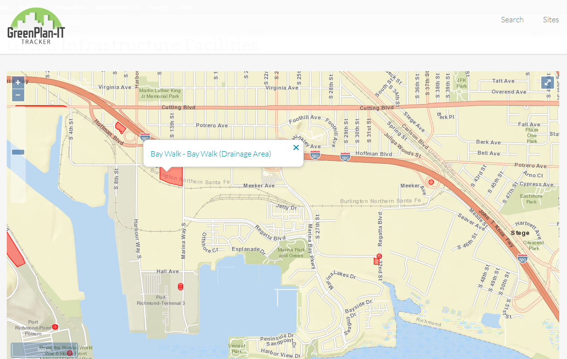
Figure 1 : The Richmond Waterfront and associated green infrastructure.
The GreenPlan-IT Tracker places green infrastructure facilities into their proper context. Figure 1 shows the Richmond waterfront with red areas marking drainage management areas associated with installed green infrastructure. Clicking on a polygon provides easy access to more information with another click.
Key Functions and Features
Detailed Information on a per-site basis

Figure 2: Detailed Information on facilities.
The tool records and displays critical information about the outputs of city planning and GI implementation for each installed facility. This includes specifics regarding the type, configuration, and geospatial information. It also records maintenance and monitoring logs that can be accessed from field locations: a key feature to help ensure that the installed facilities and the associated municipal expenditures continue to provide the value back to the community as designed.
Geospatial capabilities
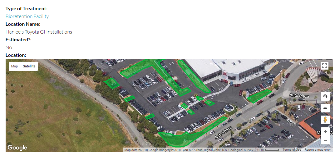
Figure 3: Detailed geospatial designation of drainage management areas and treatment areas.
The Tracker offers the ability to generate polygons in the browser, associated with drainage management areas and treatment areas. These designated areas help to determine the effect of the GI facility when also combined with its type of treatment, the configuration of its associated features, and the location in the subwatershed.
Reporting information for inclusion in stormwater reports
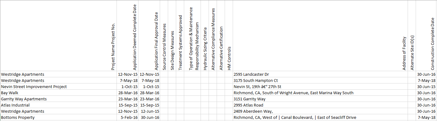
Figure 4: Information suitable for inclusion in stormwater reports.
The information stored in GreenPlan-IT reflects the information reported for individual green infrastructure facilities reported under the Provision C.3 of the Municipal Regional Permit, requiring the reporting of new development and redevelopment for regulated and special projects.
“Effectiveness reporting” for individual installations

Figure 5: Effectiveness Reporting by individual facility.
The system calculates effectiveness for individual installations. The system also calculates effectiveness on the basis of the type of green infrastructure, its specific design configuration, and its location. These factors are used to generate the effectiveness view on a per-site basis, as processed by EPA’s SWMM model in the modeler tool component, and then displayed on individual sites
Figure 5 above illustrates some sample effectiveness output. “Baseline,” in this figure, represents the estimated metrics without any GI. The columns showing “With LID” account for the effect of the individual facility. The calculated information displayed is influenced by the type of facility / BMP /LID, the details of its configuration (usually established for each green infrastructure type county-wide), and its specific location within the watershed. The SWMM model processes these inputs to determine how much infiltration of stormwater is increased and how much PCB would be removed with and without the given facility. Further information on any of the displayed items is available by hovering over the items.
“Effectiveness reporting” for the municipal green infrastructure portfolio

Figure 6: Effectiveness Reporting by jurisdiction.
Similar to the modeling based on individual facilities, the system also calculates effectiveness for the entire municipal jurisdiction on the basis of the city’s green infrastructure portfolio. The individual types of green infrastructure, their specific configurations, and their locations are collectively taken together and then processed by EPA’s SWMM model in the modeler tool of the toolkit, which employs an algorithm to calculate the collective effectiveness, which are the outcomes identified by the community in attenuating stormwater flow and filtering pollutants.
This jurisdictional view in figure 6 offers a very unique sense of the growing portfolio. The years mark the completion dates for construction of the individual green infrastructure facilities. This effectiveness reporting fosters understanding of the value of the city’s managed portfolio through a line chart that measures the increasing number of acres treated as the impervious landscape becomes more porous. Viewers, including community members and resource planners, can measure the contribution to the city’s overall attenuation of stormwater flow and pollutant load reduction in alignment with the city’s goals and permit requirements.
Mapping of sites for external use
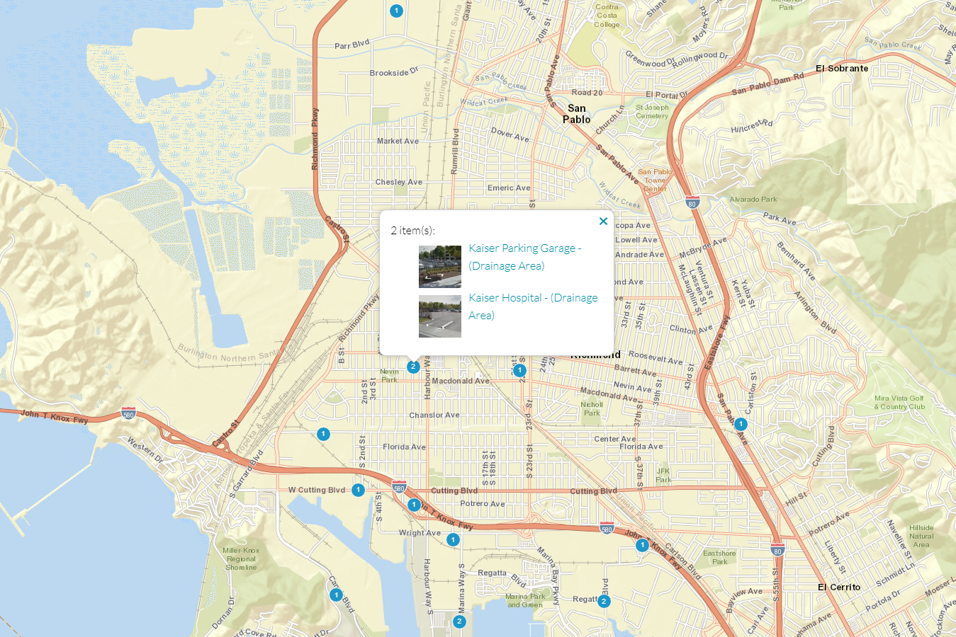
Figure 7: Embeddable map of the City of Richmond.
Sites entered into the system can be displayed by the municipality on dynamic Tracker maps that can, in turn, be embedded into the municipal website pages, staff reports, quarterly reports to the council, or any other regular reporting requirements to show the value, the outcomes of the city’s investment in green infrastructure.
Importing and exporting
Figure 8: List of sites with link to export data.
Importing new records about additions and changes to new or upgraded facilities is accomplished by entering data into the available forms. Or data can be provided to the tool’s stewards, SFEI, for reformatting and integration.
Exporting data is available for a given jurisdiction. After narrowing a list of sites to those in a selected jurisdiction, you may download the associated data, or transfer it to other platforms or data management systems as illustrated in figure 8. (You must have permission to view the data to be displayed.)
Mobile-enabled entry and editing
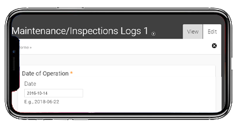
Figure 9: Mobile view of Maintenance and Inspection Logs
Responsive design allows technicians in the field to view, enter, and update information on their tablets or phones.
Licensing Plan

The Tracker is slightly different from the other modules in the GreenPlan-IT toolset. The Site Locator Tool, Modeler, and Optimizer are sophisticated, downloadable tools designed to help municipalities plan and assess their green infrastructure investments. They are freely available on the GreenPlan-IT website: http://greenplanit.sfei.org. Unlike other modules within the GreenPlan-IT toolset, the Tracker is not able to be distributed since it follows a software-as-a-service model. Its value lies in its accessibility as an easy-to-use, always-available centralized website and database.
To make GreenPlan-IT Tracker accessible to even the most budget-constrained municipality, we have scaled the cost for ongoing support and maintenance of the toolset to the number of sites entered into Tracker by the municipality. In other words, the fewer the sites the municipality has in its portfolio of installed green infrastructure, the lower its licensing costs.
The licensing fees will cover costs for hardware (server and networking equipment), bandwidth, software upgrades, basic application enhancements, and customer support.
The tiers for ongoing support are as follows:
- 1-100 Sites: $1,000 / year
- 101-500 Sites: $2,000 / year
- 501-2000 Sites: $3,000 / year
- 2001 - 5000 Sites: $4,500 / year
- > 5000: $6,000 / year
In this way, a relatively meager investment is leveraged at great value to the users and the communities they serve. The team will work with municipal managers to re-assess the licensing fees on an annual basis to ensure that a fair value is delivered.
Roadmap
This licensing structure supports the Tracker tool’s upgrades as necessary and the team’s availability to attend to user needs beyond the term of the EPA-funded contract. While we can forecast which needs might arise, we cannot always predict with great accuracy which should receive immediate attention. However, based on feedback received and opportunities already identified, what follows is a forecast of further development for the GreenPlan-IT Tracker.
Client-Base Expansion
With interest in GreenPlan-IT remaining high, the SFEI team plans for continued growth of the Tracker tool, along with the Site Locator, Modeler, and Optimizer.
Cities will continue to use Tracker to record additional sites and leverage the output for reporting. The team will support additional cities who wish to avail themselves of these features. Cities might also test their assumptions about the effectiveness of their managed portfolio of green infrastructure against the SWMM-based modeling output available to them. As implementation expands beyond the cities already using the tool, we can anticipate changes to the tool. It is designed to be extensible to customization as needs are expressed by the user base. Those changes might include some of the following ideas:
Customized Charting
The charts available to users of the tool are solid but limited. We anticipate that cities may wish to develop their own items to be charted based on as-yet-to-be determined factors.
Regional Analysis
With additional cities contributing to the Tracker, analyses conducted beyond the individual counties will be possible. The calculations for effectiveness at a more regional scale can be added to aid local decision makers who may wish to coordinate efforts at a broader scale.
Additional Modeling
The SWMM-based modeling integrated into the Tracker is a useful addition. It exposes a handful of calculations deemed to be useful to stewards of the green infrastructure. However, there are additional materials that can be calculated, shared, and visualized within the tool.
Project: Healthy Watersheds, Resilient Baylands
Another project funded by EPA’s Water Quality Improvement Fund, “Healthy Watersheds, Resilient Baylands,” will address opportunities near the Bay’s edge to address water quality needs through the use of ecologically focused solutions. GreenPlan-IT will be enhanced within this project to deliver ecologically informed hydrologic assessments of the urban landscape. At the same time, there are other project proposals in the works that may yield new enhancements for the Toolset.
Technical Specifications
The system includes primary data sources, imported or manually inputted into the system. In figure 11 below, this information falls under “Direct Inputs.” This directly contributed information is available for output via exports. The system also features information calculated or derived from the primary data, using them as inputs to a model, designed to determine the overall effectiveness, the outcomes of the green infrastructure portfolio in relation to the City's goals and permit requirements. This information is termed “Derived Outputs” in the figure below because it is the result of processing the accumulated raw data that the tool stores and turning it into the needed information for reporting out on monthly, quarterly or annual time intervals to city departments, community groups, regulators and the city council.
Figure 11: Conceptual ERD for GreenPlan-IT Tracker.
The ERD is conceptual in the context of the database because the content management system is non-normalized. It does not adhere to the conventional standards of a database designed specifically for this purpose. This allows the database versatility and adaptability. The section dedicated to effectiveness reporting does describe a more conventional normalized database model. In either case, we do document the fields nevertheless in the following collection of resources.
Platform
The Tracker is designed using open-source tools to minimize software and maintenance costs, while affording the greatest possible transparency. Documented below are the specifications for the operating system, application, scripts, database, and data structures.
Primary Application
- Operating system: Ubuntu
- Database: Postgres
- Content management system: Drupal
- Geospatial engine: PostGIS
- Geospatial visualization: OpenLayers
The primary application permits role-based security by virtue of the Drupal content management system (CMS). PostGIS and Openlayers, working together, offer geospatial enhancements to the CMS that offer advanced in-browser feature editing. The native reporting features offer sustainable and customizable reporting outputs.
Effectiveness Reporting Submodule
- Operating system: Ubuntu
- Database: Postgres
- Scripting Language: Python
- Modeling engine: SWMM5
Summary of effectiveness reporting processing
One novel innovation of the GreenPlan-IT Tracker is the integration of EPA’s SWMM5 model into the Tracker online database. The scripts are written in Python using a wrapper to call the EPA's SWMM5 model (https://pypi.org/project/SWMM5/). An unmodified version of SWMM5 handles all of the analysis. Meanwhile, the Python-based wrapper code manages the tasks, dynamically modifying a template SWMM input file, triggering SWMM via the wrapper library, parsing the output file, and updating the analytical database.
Detailed description
The processing proceeds in this fashion on a daily basis:
- Tasks are stored in the GPT database when any node is modified by Drupal (using short Drupal module written in PHP)
- Python, when run, retrieves the list of queued tasks from the database
- Duplicate tasks or tasks with insufficient input data are marked as such and ignored
- For each valid task, Python queries the database to get relevant input data, then modifies a "template" SWMM5 input file (just formatted text really). The template being manually created for each region/jurisdiction.
- The wrapper triggers SWMM5 to run using that modified input file and Python waits for it to finish.
- Once finished, Python parses the output report file (just formatted text), then uploads the relevant data back into the GPT database.
- The regional tasks are run similarly, except instead of just using one node to modify the input, it uses all the nodes within the jurisdiction.
Field specs
Primary Application
Watershed Characteristics
- TABLE: Watershed Identification
- Watershed_ID
- Char
- 24
- Watershed_Name
- Char
- 256
- Watershed_ID
Socio - Economic Characteristics
- TABLE: Site_Location
- City
- Char
- 60
- County_Code
- Char
- 5
- State_Code
- Char
- 2
- Zip
- Char
- 14
- Geocode_Latitude
- Char
- 10
- Geocode_Longitude
- Char
- 11
- Reference_Datum (Horizontal)
- Char
- (e.g., NAD83, WGS84)
- City
LID Characteristics
- TABLE: Identification
- Title
- Char
- 256
- Alternate_Site ID(s)
- Char
- 24
- Alternative_Certification
- Char
- 24
- Alternative_Compliance_Measures
- Char
- 24
- Description
- Char
- Long
- Name_of_Developer
- Char (Validated)
- 24
- Public/Private
- Char (Validated)
- 24
- Status
- Char (Validated)
- 24
- Total_Area_of_Land_Disturbed (Acres)
- Num
- Total_New_Impervious_Surface_Area (ft2)
- Num
- Total_PostProject_Impervious_Surface_Area (ft2)
- Num
- Total_PreProject_Impervious_Surface_Area (ft2)
- Num
- Total_Replaced_Impervious_Surface_Area (ft2)
- Num
- Total_Site_Area (Acres)
- Num
- Title
- TABLE: GI_feature_area
- Associated_LID_ID
- Char
- 24
- Geometry
- Char
- Long
- Location
- Binary
- KML
- Latitude
- Double
- Feature Centroid
- Longitude
- Double
- Feature Centroid
- Area
- Num
- Reference_Datum (Horizontal)
- Associated_LID_ID
- TABLE: Owner_Information
- Owner_type
- Char
- 24
- Owner_Name
- Char
- 50
- Owner_Contact
- Char
- 50
- Owner_type
- TABLE: Drainage_management_area
- Type_of_Treatment_HM_Controls_Inspected
- Char
- 24
- Location_Name
- Char
- 256
- Estimated
- Char
- 24
- Geometry
- Char
- Long
- Location
- Binary
- KML
- Latitude
- Double
- Longitude
- Double
- Reference_Datum (Horizontal)
- Type_of_Treatment_HM_Controls_Inspected
Design Characteristics
- TABLE: Infiltration_rates
- Capacity
- Num
- filter_rate
- Num
- Designed_to_Hold_Water_72_Hours
- Char
- 24
- Capacity
- TABLE: Soil_media
- Type
- Char
- 24
- Depth
- Num
- Num
- Type
- TABLE: Permitting_process
- Application_Deemed_Complete_Date
- Date
- Application_Final_Approval_Date
- Date
- Construction_Complete_Date
- Date
- Application_Deemed_Complete_Date
Costs
- TABLE: LID_costs
- Installation_cost
- Num
- Mainanence_cost
- Num
- Rehabilitation_cost
- Num
- Installation_cost
Maintenance Information
- TABLE: Event_Maintenance
- LID_ID
- Char
- 24
- Date
- Date
- Type_of_Operation_Inspection
- Char
- 24
- Inspection_Findings_or_Results
- Char
- Long
- Enforcement_Action_Taken
- Char
- Long
- Comments_Follow-up
- Char
- Long
- Activity
- Char
- Long
- Outcome
- Char
- Long
- Status
- Char
- 24
- LID_ID
Reports / Engineered Drawings
- TABLE: File_Attachments
- File_Attachment
- Binary
- Comments
- Char
- Long
- Date
- Date
- File_Attachment
Lookup Tables
TABLE: LID_Types
|
Code |
Description |
|
biornu |
Bioretention without an Underdrain |
|
biorwu |
Bioretention with an Underdrain |
|
ftpb |
Flow Through Planter Box |
|
inft |
Infiltration Trench |
|
prpv |
Permeable Pavement |
|
swwt |
Stormwater Wetland |
|
trbx |
Tree Box |
|
vgsw |
Vegetated Swale |
|
wtpd |
Wet Pond |
TABLE: Maintenance_Status
|
Code |
Description |
|
NM |
needs maintenance |
|
GC |
good condition |
|
SM |
scheduled for maintenance |
TABLE: Owner_type
|
Code |
Description |
|
CNG |
County Government |
|
COR |
Corporation |
|
CTG |
Municipality |
|
DIS |
District |
|
FDF |
Federal Facility (U.S. Government) |
|
GOC |
GOCO (Gov Owned/Contractor Operated) |
|
IND |
Individual |
|
MWD |
Municipal or Water District |
|
MXO |
Mixed Ownership (e.g., Public/Private) |
|
NON |
Non-Government |
|
POF |
Privately Owned Facility |
|
SDT |
School District |
|
STF |
State Government |
|
TRB |
Tribal Government |
|
UNK |
Unknown |
Effectiveness Reporting Submodule
The effectiveness reporting subsystem leverages EPA’s SWMM5 model to calculate a number of key outputs from the data within the system. The tables below are discrete from the functions associated with the general tracker application since these tables are specialized to hold SWMM-based parameters, input data, and output data.
Task tables
- TABLE: task
Table of all SWMM tasks. Populated by drupal on node update hook. Updated and run (or declined) by Python/SWMM scripts.
- taskid
- Integer
- Unique, non-null, primary key
- Autofill, sequential
- nodeid
- Integer
- Statuscode
- Text
- Matches key “statuscode” in table “statuslu”
- Only used when linked to regional tasks to track total treated drainage management area in regional run
- requestdate
- Timestamp
- processdate
- Timestamp
- finishdate
- Timestamp
- modelversion
- Text
- totaldma
- Integer
- TABLE: regionaltask
A table for tracking regional tasks, that is, a task aggregating a whole region (as opposed to individual GI installation). Does not track the model task itself, but each entry is linked to a task in the task table.
- regiontaskid
- Integer
- Unique, non-null, primary key
- Autofill, sequential
- regionid
- Integer
- Matches key “regionid” in table “regionlu”
- taskid
- Integer
- Matches key “taskid” in table “task”
- statuscode
- Text
- Matches key “statuscode” in table “statuslu”
- taskyear
- Integer
- tasktype
- Text
- To identify task if not by year (usually ‘baseline’ task or ‘all’ task)
- lasttaskid
- Integer
- Matches key “taskid” in table “task”
- Last completed task id if new task in queued or processing
Output Tables
- TABLE: runoffoverview
Summary of runoff quantity continuity. Will only be one row per task.
- runoffoverviewid
- Integer
- Unique, non-null, primary key
- Autofill, sequential
- taskid
- Integer
- Matches “taskid” in table “tasks”
- initiallidstorage
- Float
- Acre-feet
- evaporationloss
- Float
- Acre-feet
- infiltrationloss
- Float
- Acre-feet
- surfacerunoff
- Float
- Acre-feet
- finalstorage
- Float
- Acre-feet
- continuityerror
- Float
- totalprecipitation
- Float
- Acre-feet
- TABLE: pollutantoverview
Summary of runoff quantity continuity for pollutants. One row per task per pollutant tracked (which for now is only PCB).
- pollutantoverviewid
- Integer
- Unique, non-null, primary key
- Autofill, sequential
- taskid
- Integer
- Matches “taskid” in table “tasks”
- pollutant
- Text
- We only track PCB so value here will only be that, but leaving flexible in case that changes in the future
- initialbuildup
- Float
- Values in lbs (at least for PCB, only output we track for now)
- surfacebuildup
- Float
- Values in lbs (at least for PCB, only output we track for now)
- wetdeposition
- Float
- Values in lbs (at least for PCB, only output we track for now)
- sweepingremoval
- Float
- Values in lbs (at least for PCB, only output we track for now)
- Infiltrationloss
- Float
- Values in lbs (at least for PCB, only output we track for now)
- bmpremoval
- Float
- Values in lbs (at least for PCB, only output we track for now)
- surfacerunoff
- Float
- Values in lbs (at least for PCB, only output we track for now)
- remainingbuildup
- Float
- Values in lbs (at least for PCB, only output we track for now)
- continuityerror
- Float
- TABLE: runoff
Detailed runoff statistics. This and following tables designed to handle multiple rows per task, for each LID, for each subcatchment, or combination thereof as necessary.
- runoffid
- Integer
- Unique, non-null, primary key
- Autofill, sequential
- taskid
- Integer
- Matches “taskid” in table “tasks”
- subcatchmentid
- Integer
- Matches “id” in table “subcatchments”
- I don’t think region_id is needed since subcatchment_id should be unique itself
- totalprecipin
- Float
- Inches
- totalevapin
- Float
- Inches
- totalinfilin
- Float
- Inches
- totalrunoffin
- Float
- Inches
- totalrunoffgal
- Float
- Gallons (technically SWMM outputs in mega-gallons, note to self, either convert before storing value or be sure to note it’s not in straight gallons)
- peakrunoffcfs
- Float
- CFS
- runoffcoeff
- Float
- TABLE: lidperformance
Detailed LID statistics.
- lidperformanceid
- Integer
- Unique, non-null, primary key
- Autofill, sequential
- taskid
- Integer
- Matches “taskid” in table “tasks”
- subcatchmentid
- Integer
- Matches “subcatchmentid” in table “subcatchments”
- lidtype
- Text
- totalinflowin
- Float
- Inches
- evaplossin
- Float
- Inches
- infillossin
- Float
- Inches
- surfaceoutflowin
- Float
- Inches
- drainoutflowin
- Float
- Inches
- initialstoragein
- Float
- Inches
- finalstoragein
- Float
- Inches
- continuityerror
- Float
- TABLE: washoff
Detailed washoff statistics.
- washoffid (need better name)
- Integer
- Unique, non-null, primary key
- Autofill, sequential
- taskid
- Integer
- Matches “taskid” in table “tasks”
- subcatchmentid
- Integer
- Matches “subcatchmentid” in table “subcatchments”
- pcblbs
- Float
- PCB in lbs
- May potentially be more columns for other pollutant types, but would follow same format (for now PCBs are only ones we track)
Lookup tables (and also subcatchment)
- TABLE: statuslu
Status types (e.g. “Processing”, “Declined”, “Error”).
- statuscode
- Text
- Unique, non-null, primary key
- statusname
- Text
- statusdesc
- Text
- TABLE: regionlu
Regions for different jurisdictions and/or SWMM model input. Right now should only hold “Richmond”.
- regionid
- Integer
- Unique, non-null, primary key
- regionname
- Text
- regiontid
- Integer
- TID for jurisdiction as tracked in Drupal
- TABLE: subcatchment
Watershed subcatchment geometries.
- subcatchmentid
- Integer
- Unique, non-null, primary key
- subcatchmentname
- Text
- regionid
- Integer
- Matches key “regionid” in table “regionlu”
- geom
- Geometry (EPSG 3310)

Contact
Contact us with any questions, feedback, or problems. Please let us know if you have any questions about the GreenPlan-IT Toolset or this site.
Send us an email: tech@sfei.org
Documentation
The following pages represent deprecated content that may nevertheless be a valuable reference to you as you implement GreenPlan-IT in your municipality.
Latest Reports
Report
Zi, T.; Whipple, A.; Kauhanen, P.; Spotswood, E.; Grenier, L.; Grossinger, R.; Askevold, R. 2021. Trees and Hydrology in Urban Landscapes. SFEI Contribution No. 1034. San Francisco Estuary Institute: Richmond, CA.
 Effective implementation of urban greening strategies is needed to address legacies of landscape change and environmental degradation, ongoing development pressures, and the urgency of the climate crisis. With limited space and resources, these challenges will not be met through single-issue or individual-sector management and planning. Increasingly, local governments, regulatory agencies, and other urban planning organizations in the San Francisco Bay Area are expanding upon the holistic, portfolio-based, and multi-benefit approaches.
This effort, presented in the Trees and Hydrology in Urban Landscapes report, seeks to build links between stormwater management and urban ecological improvements by evaluating how complementary urban greening activities, including green stormwater infrastructure (GSI) and urban tree canopy, can be integrated and improved to reduce runoff and contaminant loads in stormwater systems. This work expands the capacity for evaluating engineered GSI and non-engineered urban greening within a modeling and analysis framework, with a primary focus on evaluating the hydrologic benefit of urban trees. Insights can inform stormwater management policy and planning.
Journal Article
Wu, J.; Kauhanen, P.; Hunt, J. A.; Senn, D.; Hale, T.; McKee, L. J. . 2019. Optimal Selection and Placement of Green Infrastructure in Urban Watersheds for PCB Control. Journal of Sustainable Water in the Built Environment 5 (2) . SFEI Contribution No. 729.
Optimal Selection and Placement of Green Infrastructure in Urban Watersheds for PCB Control.
San Francisco Bay and its watersheds are polluted by legacy polychlorinated biphenyls (PCBs), resulting in the establishment of a total maximum daily load (TDML) that requires a 90% PCB load reduction from municipal stormwater. Green infrastructure (GI) is a multibenefit solution for stormwater management, potentially addressing the TMDL objectives, but planning and implementing GI cost-effectively to achieve management goals remains a challenge and requires an integrated watershed approach. This study used the nondominated sorting genetic algorithm (NSGA-II) coupled with the Stormwater Management Model (SWMM) to find near-optimal combinations of GIs that maximize PCB load reduction and minimize total relative cost at a watershed scale. The selection and placement of three locally favored GI types (bioretention, infiltration trench, and permeable pavement) were analyzed based on their cost and effectiveness. The results show that between optimal solutions and nonoptimal solutions, the effectiveness in load reduction could vary as much as 30% and the difference in total relative cost could be well over $100 million. Sensitivity analysis of both GI costs and sizing criteria suggest that the assumptions made regarding these parameters greatly influenced the optimal solutions.
City Engagements
City of Sunnyvale
Wu, J., Kauhanen, P., Hunt, J.A., and McKee, L.J., 2018. Green Infrastructure Planning for the City of Sunnyvale with Greenplan-IT. A joint technical report of the Environment Informatics Program and the Clean Water Program. Contribution No. 881. San Francisco Estuary Institute, Richmond, California. https://www.sfei.org/
City of Richmond
Wu, J., Kauhanen, P., Hunt, J.A., and McKee, L.J., 2018. Green Infrastructure Planning for the City of Richmond with Greenplan-IT. A joint technical report of the Environment Informatics Program and the Clean Water Program. Contribution No. 883. San Francisco Estuary Institute, Richmond, California. https://www.sfei.org/
City of Oakland
Wu, J., Kauhanen, P., Hunt, J.A., and McKee, L.J., 2018. Green Infrastructure Planning for the City of Oakland with Greenplan-IT. A joint technical report of the Environment Informatics Program and the Clean Water Program. Contribution No. 884. San Francisco Estuary Institute, Richmond, California. https://www.sfei.org/
North Richmond
Wu, J., Kauhanen, P., Hunt, J.A., and McKee, L.J., 2018. Green Infrastructure Planning for North Richmond Pump Station Watershed with Greenplan-IT. A joint technical report of the Environment Informatics Program and the Clean Water Program. Contribution No. 882. San Francisco Estuary Institute, Richmond, California. https://www.sfei.org/
East Bay Corridor
Kauhanen, P., Wu, J., Hunt, J.A., and McKee, L.J., 2018. Green Plan-IT Application Report for the East Bay Corridors Initiative. A joint technical report of the Environment Informatics Program and the Clean Water Program. Contribution No. 887. San Francisco Estuary Institute, Richmond, California. https://www.sfei.org/
GreenPlan-IT Toolkit Demonstration Report
GreenPlan-IT Toolkit Demonstration Report
Prepared by
SAN FRANCISCO ESTUARY INSTITUTE
4911 Central Avenue, Richmond, CA 94804
Phone: 510-746-7334 (SFEI)
Fax: 510-746-7300
www.sfei.org

Table of Contents
1.1. Project Rationale
1.2. Overview of GreenPlan-IT Toolkit
1.3. GreenPlan-IT Toolkit Application Process
Chapter 2. Case Study: City of San Mateo
2.1 Project setting
2.2 Data layers collected and used for locator tool
2.3 Site Locator tool setup
2.4 Results Analysis
Chapter 3. Case Study: San Jose Priority Development Area
3.1 Project Setting
3.2 GIS Site Locator Tool
- Data layers collected and used
- Site Locator tool setup
- Results Analysis
- Ranking of sites
- Expected/desired final product
- Final steps to get all results to 100% (maps)
3.3 Modeling Tool
3.3.1 Data Collection
3.3.2 Model Setup
3.3.3 Model Calibration
3.3.4 Baseline Condition
3.4 Optimization Tool
3.4.1 Focus Area
3.4.2 Optimization Problem Formulation
3.4.3 Design Storm
3.4.4 GI Representation
3.4.5 GI Cost
3.4.6 Optimization Results
3.4.7 Sensitivity Analysis
Chapter 4. Discussion and Recommendations
4.1 Lessons learned
4.2 Data Gaps
4.3 Future steps/enhancement
Executive Summary
GreenPlan-IT is a planning level tool that was developed by SFEP and SFEI with support and oversight from BASMAA to provide Bay Area municipalities with the ability to evaluate multiple management alternatives using green infrastructure for addressing stormwater issues in urban watersheds. GreenPlan-IT combines sound science and engineering principles with GIS analysis and optimization techniques to support the cost-effective selection and placement of Green Infrastructure (GI) at a watershed scale. Tool outputs can be used to develop quantitatively-derived watershed master plans to guide future GI implementation for improving water quality in the San Francisco Bay and its tributary watersheds.
Structurally, the GreenPlan-IT is comprised of three components: (a) a GIS-based Site Locator Tool to identify potential GI sites; (b) a Modeling Tool that quantifies anticipated watershed-scale runoff and pollutant load reduction from GI sites; and (c) an Optimization Tool that uses a cost-benefit analysis to identify the best combinations of GI types and number of sites within a watershed for achieving flow and/or load reduction goals. The three tool components were designed as standalone modules to provide flexibility and their interaction is either through data exchange, or serving as a subroutine to another tool.
This report provides an overview of the GreenPlan-IT Tool and demonstrates its utility and power through two pilot studies which is summarized in this report as a case study. The pilot studies with the City of San Mateo and the City of San Jose explored the use of GreenPlan-IT for identifying feasible and optimal GI locations for mitigation of stormwater runoff. They are provided here to give the reader an overview of the user application process from start to finish, including problem formulation, data collection, GIS analysis, establishing a baseline condition, GI representation, and the optimization process. Through the pilot study application process the general steps and recommendations for how GreenPlan-IT can be applied and interpreted are presented.
The pilot with the City of San Mateo utilized only the GIS Site Locator Tool to screen potential sites for GI implementation in five discrete watersheds (Borel Creek, Laurel Creek, Leslie Creek, Poplar Creek, San Mateo Creek) as well as multiple unnamed drainages. Using selected regional and local data layers and the City’s ranking and weighting and using all five optional analyses, the Site Locator Tool identified 18 acres of City-owned property or right-of-way as highly ranked locations for potential GI implementation, 113 acres as moderately ranked, and 11 acres as lower ranked locations. A remote data vaGIation exercise confirmed that many of the sites identified and ranked highly by the locator tool were also sites previously identified as potential GI opportunities by the city of San Mateo.
The pilot study with City of San Jose used the full Toolkit to support a cost-benefit evaluation of stormwater runoff control. The objective of this pilot was to demonstrate the capacities and usability of GreenPlan-IT for identifying feasible and cost-effective GI locations at a watershed scale. The focus area was a 4300 acre proposed development area within the lower part of the Guadalupe River Watershed. The Site Locator Tool identified possible GI locations that serve as the constraints for the optimization process; the Modeling Tool established a representative baseline condition through calibration to local data; and then the Optimization Tool was used to repeatedly run the Modeling Tool to iteratively arrive at the optimized GI scenario that minimized the total cost of management while satisfying water quality and quantity constraints. The results of the application included the cost/benefit associated with a range of flow or loads reduction targets, ranking of sites for specific optimal solutions, and maps showing the distribution of GI within the study area under a specific optimal solution.
The Site Locator Tool has end-user flexibility that results in an iterative tool that can be fine-tuned as questions and goals change or more accurate local data are available. Establishing a representative baseline model is crucial for meaningful results and requires the calibration of the Modeling Tool to local data. The Optimization Tool can be very powerful when combined with hydrologic modeling and cost analyses. Successful and meaningful application of the Optimization Tool largely depends on accurate representation of the watershed baseline condition, GI configurations, and the associated GI costs. The cost-effective solutions from the optimization process must be interpreted in the context of specific problem formulation, assumptions, constraints, and optimization goals unique to each application. With the help of this information, decision makers can set realistic goals on how much can be achieved and the level of investment required, as well as determine at what point further investment on GI will yield no improvement in runoff reduction.
Introduction
Chapter 1
Water quality in the San Francisco Bay and its watersheds is impaired by PCBs, mercury, pesticides and a number of other pollutants associated with stormwater runoff. Reducing stormwater runoff and contaminant loads is complex and relies on costly engineering, especially in highly-developed urban environments. Increasingly, distributed management of stormwater runoff using Green infrastructure (GI) is emerging as a multi-benefit solution that can address both stormwater quality and quantity concerns. Consistent with this trend, and under anticipated new stormwater permit provisions due in 2015, Bay Area local governments will be required to develop and implement watershed-scale green infrastructure plans to achieve quantitative water quality improvements.
A major barrier to regional-scale, widespread implementation of GI is a lack of watershed-based planning regarding where opportunity sites exist for GI retrofits and what constitutes the most cost-effective, achievable, and practical management strategy for achieving water quality targets for local landscapes. Realizing the need for a planning tool to support Bay Area municipalities to strategically plan and implement GI projects at a watershed scale, the State Board funded a research project[1] to develop a Toolkit that meets technical and institutional requirements for successful selection and implementation of GI projects. The resulting Toolkit was branded “GreenPlan-IT”. The Toolkit package, consisting of the software, companion user manuals, and this demonstration report, is available on the GreenPlan-IT Web site hosted by SFEI (http://greenplanit.sfei.org/).
This report describes the rationale for developing the GreenPlan-IT Toolkit; explains the Toolkit’s design and structure; and demonstrates the Toolkit’s capabilities through two case studies. Where appropriate, this report also examines the limitations of the Toolkit and provides recommendations for future enhancements. The additional input data/outputs for the Toolkit are also included in the appendices.
1.1 Project Rationale
Surface water degradation resulting from stormwater runoff has been an issue of primary focus for many Bay Area agencies. Despite the recognized effectiveness of GI in protecting water quality and reducing flood risk, and the mandatory implementation of GI under limited circumstances under the current NPDES Stormwater Municipal Regional Permit (MRP), the Bay Area’s implementation of GI continues slowly. To date, GI projects are largely placed opportunistically (e.g., where land becomes available), or as demonstration projects, at different points throughout a drainage area, with unknown and likely suboptimal flow and load reduction effectiveness. Little is known about the cumulative effects of implementing hundreds or even thousands of GI projects in Bay Area watersheds, either alone or in well-planned combination with “grey infrastructure” approaches. In addition, future MRPs will likely require local agencies to implement GI to achieve set goals at the watershed scale. Bay Area agencies need a scientifically sound planning tool to help develop quantitatively-derived watershed master plans to guide future GI implementation for improving water quality in the San Francisco Bay and its tributary watersheds.
GreenPlan-IT was developed to meet this critical need. The Toolkit can facilitate identification, evaluation and ranking of potential sites based on their relative feasibility and potential effectiveness in reducing stormwater runoff and pollutant loads. GreenPlan-IT can help Bay Area municipalities to address the following key stormwater management questions:
- Where are the suitable locations for GI implementation within the built-out urban environment?
- Where are the effective locations for GI implementation that could have the greatest potential leverage or effectiveness for reducing peak flow runoff and contaminant loads?
- What quantitative water quality and hydrological improvements can be made with GI approaches?
- What are the most cost-effective GI combinations for achieving certain reduction targets?
GreenPlan-IT combines a GIS screening tool, a publically available modeling platform, and an Optimization Tool to provide users with the ability to evaluate multiple stormwater management alternatives to support their decision making for addressing a variety of issues. The Toolkit can be used to comply with NPDES stormwater permit requirements including the development of an alternative compliance program, as well as addressing loads reduction needs identified in TMDLs. The Toolkit is intended for knowledgeable users familiar with GI and the technical aspects of watershed modeling, and applicable to predominantly urban watersheds. Although designed as a tool for Bay Area stormwater agencies, the tool has broad applicability and could be used by other regions as well.
1.2 Overview of GreenPlan-IT Toolkit
The GreenPlan-IT Toolkit is designed to support the cost-effective selection and placement of GI in urban watersheds through GIS analysis, hydrologic modeling and optimization techniques. The Toolkit consists of three components: GIS Site Locator Tool, Modeling Tool, and Optimization Tool. To provide flexibility for the user community and for future updates, the three components were designed as standalone modules and their interaction is either through data exchange, or as a submodule linked to another tool component. Figure 1-1 shows a generalized schematic of the Toolkit. Each tool in the Toolkit performs specific functions and is typically applied in sequence.
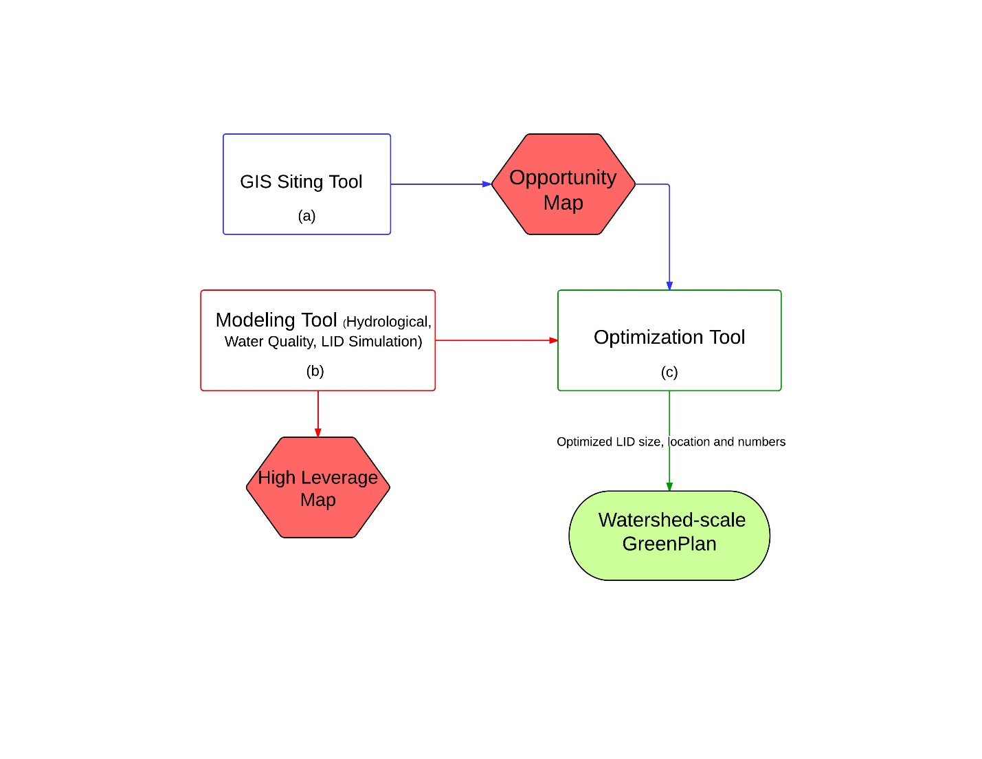
Figure 1-1. Schematic of GreenPlan-IT Toolkit
GIS Site Locator Tool
The GIS based Site Locator Tool is a screening tool that can be used to identify and rank potential GI locations through GIS analysis. The Tool incorporates many regional, publicly available data layers and builds in five intersecting analyses that require user input data to produce maps of possible GI locations. These analyses are optional, providing end-user flexibility to add local data layers to best identify suitable locations and rankings of GI locations, to produce outputs of different levels of refinement, and to run the analyses with varying levels of data availability. The Site Locator Tool can be fine-tuned iteratively as additional local data or data with better resolution become available.
There are five optional analyses within the Site Locator Tool: the Regional Base Analysis (RBA), Locations Analysis, Opportunities and Constraints Analysis, Ownership Analysis, and Knockout Analysis (Figure 1-2). The Tool can be run with any combination or all analyses provided that data are included in each of the analysis tables. Also, there are six GI feature types in the Tool: bioretention, permeable pavement, vegetated swale, stormwater wetlands, wet pond, and infiltration trench. Any combination or all feature types can be selected when running the Tool.
The Regional Base Analysis is hardcoded and can’t be modified in the Tool. However, including the Regional Base Analysis in the Tool run is optional. This analysis provides a first estimate of GI possible locations based on regional data sets including depth to groundwater, hydrologic soil type, land use, liquefaction risk, and slope. In the analysis, each regional data set is weighted to reflect relative importance for GI suitability and is binned into relevant value bins which are ranked according to suitability for each GI type. These weights and rank values are then used in a Categorical Weighted Overlay to produce maps of the most suitable areas for each GI type. Since the data are regional in nature, the map outputs are grosser in scale and may remove potential GI locations from the output. Users can experiment by running the Tool with and without the Regional Base Analysis and then compare map outputs or use the RBA in the Opportunities and Constraints Analysis in a later step.
The Locations Analysis uses regional and local data layers to identify locations for GI implementation for each GI feature type selected. Specified location layers that are identified as potential locations are unioned in order to create a single layer for each GI type that represents all potential locations for that GI type. On-street parking, sidewalks, pedestrian trails, parking lots, and parks are example locations for implementing GI. Other potentially good locations could include traffic medians, brown field lots, and undeveloped land.
The Opportunities and Constraints Analysis is an editable table where both regional and local data sets can be added. Each data set is ranked as an opportunity (rank of 1) or a constraint (rank of -1) for GI implementation. Each data layer is then categorized into factors and then individually weighted within its factor. A weight is then assigned to each factor. These values were then used to calculate a final relative rank for each location.
The Ownership Analysis allows the Tool to delineate outputs into public and private possible location. This is only possible if a local ownership data layer exists. The ownership analysis can be important for identification of potential public private partnerships. It can also provide an opportunity to grossly analyze the proportional opportunity between publicly and privately own lands.
The Knockout Analysis in the Tool excludes landscape features that should not be included for GI consideration such as wetlands, riparian areas, and tidal areas. Buffer areas can be added to these features as well.
Once GI feature types have been selected and all input tables are filled out and the analyses are selected the Tool runs through each analysis sequentially. The Regional Base Analysis takes the area of interest and excludes all regional areas that were determined not suitable for each GI type. Next, the Locations Analysis intersects the Base Analysis area with all possible GI locations that were specified for each GI type selected. This refines the output to include only locations that are possible, as determined by the Regional Base Analysis, and meet the requirements identified in the Locations Analysis. The Opportunities and Constraints Analysis then applies a relative rank for each location by preforming a nested weighted sum. The Ownership Analysis then applies specified ownership data in order to label each location as either public or private. Lastly the Knockout Analysis removes any areas that are deemed infeasible from the map output.
The Tool produces a KML (Google Earth) and Arc-GIS map with color-coded relative rank of potential GI locations. The developed maps should then be validated via an on screen or field effort to provide verification of the ability for the input data and data ranking to produce real world results. Once validated, these sites, combined with local expert unmapped information such as areas of flooding or high pollutant areas, can serve as a starting point to plan and prioritize placement of GI within a watershed. The identified sites can also be used by the Optimization Tool to construct and constrain all potential locations in order to identify most cost-effective combinations for achieving specific management targets.
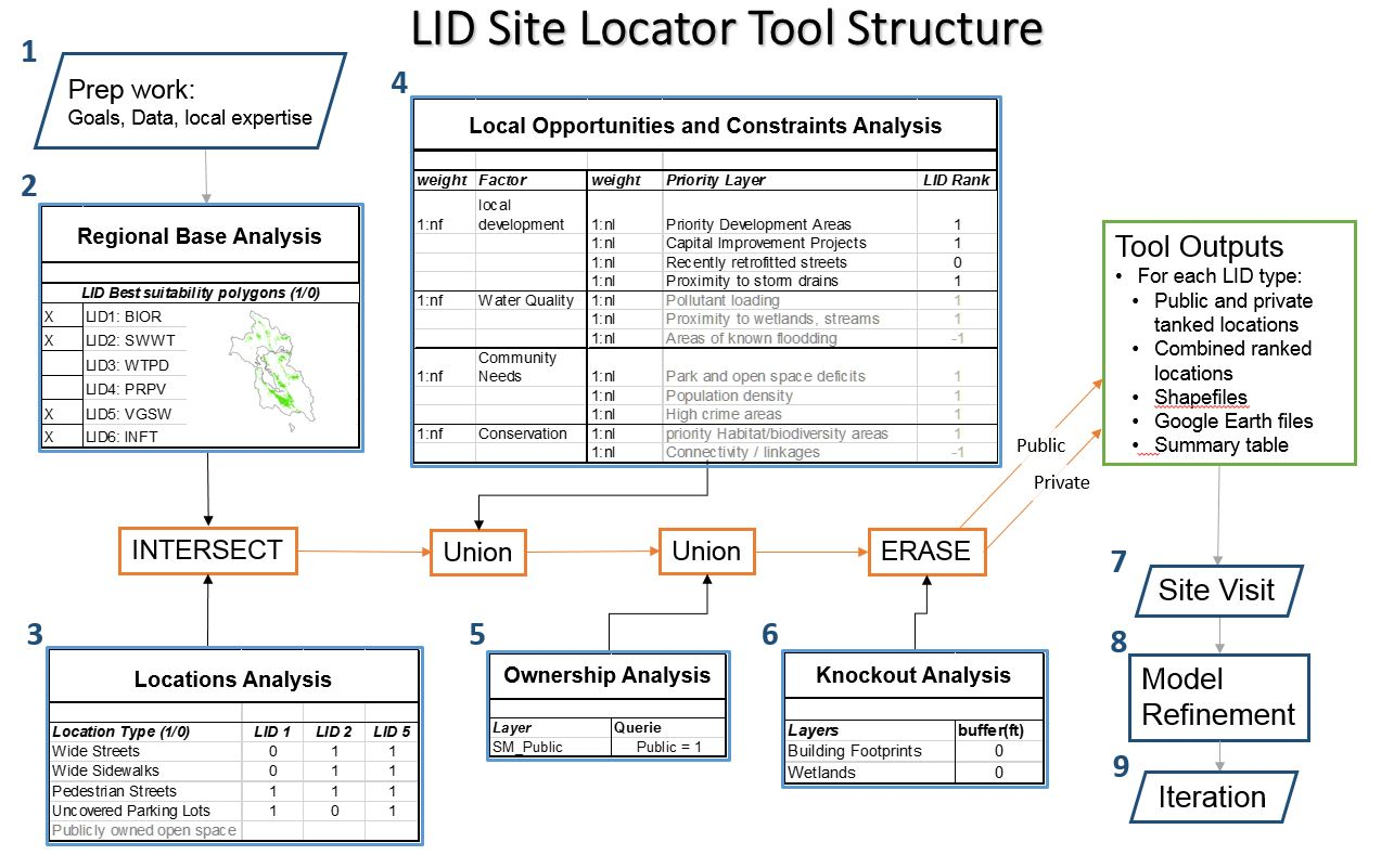
Figure 1-2. Structure of the GIS Site Locator Tool including pre-tool preparation and post tool steps.
Modeling Tool
The second tool component of the GreenPlan-IT Toolkit is built on a spatially distributed hydrologic and water quality model, EPA Storm Water Management Model (SWMM) version 5.0 (Rossman, 2010), to simulate the generation, fate and transport of stormwater runoff and associated pollutants from the landscape, as well as resulting flow and pollutant loading reduction as they pass through various GIs. The Modeling Tool is used to establish baseline conditions, identify high-yield runoff and pollution areas; and quantify any reduction made from GI implementation across different areas within a watershed. Within the Toolkit, the Modeling Tool serves as a subroutine to the Optimization Tool. At each iteration during the optimization process, the Optimization Tool will commend the Modeling tool to evaluate GI performance and pass that information back. This process progresses step by step marching towards the most cost-effective GI solutions.
Optimization tool
The third tool is an Optimization Tool which uses an evolutionary optimization technique (Non-dominated Sorting Genetic Algorithm II , Deb, et al 2002) to evaluate the benefits (runoff and pollutant load reductions) and costs associated with various GI implementation scenarios (type, location, number) and identify the most cost-effective options that satisfy user-defined management goals. The Optimization Tool requires the site information generated from the GIS Site Locator tool to form its search space, and uses the Modeling Tool as a subroutine during the search process in an iterative and evolutionary fashion to evaluate the GI performance. Therefore, using the Optimization Tool will require the running of both the Site Locator Tool and Modeling Tool.
1.3 GreenPlan-IT Toolkit Application Process
The application of the GreenPlan-IT Toolkit usually begins with the GIS Site Locator Tool, followed by the Modeling Tool, and concludes with the Optimization Tool. Since the Toolkit is constructed in a modular structure with three standalone tools, users can sometime choose to use just the GIS Site Locator Tool to do a preliminary screening on potential GI sites instead of using the full package. However, within the premise of this project, wherever possible, the application of the whole Toolkit is recommended, since optimal placement (achieving the most flow or load reduction) for the least cost is usually in the best interests of the public.
The typical step-by-step process in Toolkit application is as follows: 1) definition of study objectives; 2) data collection; 3) Toolkit setup, and 4) analysis of results. Figure1-3 is a flow diagram illustrating the Toolkit application process. The first step in the setup and application of the Toolkit is a clear definition of the study goals to ensure the most appropriate and useful application. An example of a study objective might be to identify a set of management options that achieve a required level of runoff. The study goals will define the scope and extent of the Toolkit application, including model domain, data needs, runoff and pollutant factors to be simulated, and the optimization evaluation factors and flow or pollutant load reduction targets.
The data collection for the Toolkit application involves a thorough review and compilation of data available for the study area. The Toolkit requires a variety of input data including GIS data, landscape characteristics data, GI data, and monitoring data. Table 1-1 shows a summary of typical data needs for each tool. Because the quality of the Toolkit outputs depends on the quality of input data, locally derived higher-resolution data are desired, wherever possible.
Setting up the Toolkit involves using the data collected to establish a representation of the study area. Since there is no linkage between the Site Locator Tool and Modeling Tool, they can be set up in parallel. In the case of the Modeling Tool, model calibration with local data is needed in order to ensure the establishment of a representative baseline condition. The Optimization Tool then synthesizes information from the Site Locator Tool and Modeling Tool and generates solutions that are looped back to the Modeling Tool for an iterative evaluation. Via this evolutionary search process, the most cost-effective GI solutions are identified according to the user’s specific conditions and objectives. The results of the application include the cost/benefit associated with a range of flow or loads reduction targets, ranking of sites for specific optimal solutions, and maps showing the distribution of GI within the study area under a specific optimal solution.
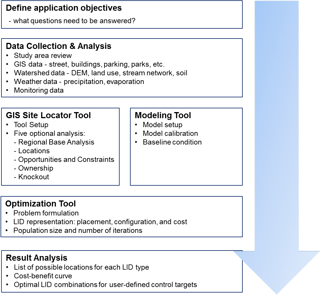
Figure 1-3. GreenPlan-IT Toolkit application process.
Table 1-1 Summary of typical data needs for the Toolkit
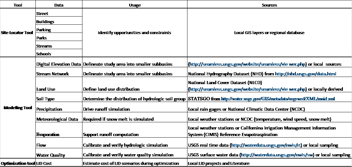
[1] Initiated by San Francisco Estuary Partnership (SFEP), San Francisco Estuary Institute (SFEI), Bay Area Storm Water Management Agencies Association (BASMAA), and partnering municipalities in 2013 through the Proposition 84 Storm Water Grant Program.
Case Study: City of San Mateo
Chapter 2
2.1 City of San Mateo’s Sustainable Street Effort
The City of San Mateo was one of two primary municipal partners in the development of the GIS Site Locator Tool. San Mateo is a city on the San Francisco Peninsula with a population of about 100,000 people. When the Green Plan Bay Area project began, the City was in the process of developing a Sustainable Streets Plan. This plan combined two other city planning efforts, a Complete Streets Plan and a Green Streets Plan, into one comprehensive plan. The Complete Streets Plan balances development and redevelopment of all modes of transportation including pedestrian, bicycle, cars, and public transportation in order to create streetscapes accessible to all transportation modes. The Green Streets Plan creates a blueprint for urban greening and returning some more natural watershed function and attributes to the cityscape. One of the primary benefits for urban greening and implementing green infrastructure is to improve the water quality of stormwater runoff that drains to the Bay. In addition, the City also desired other green infrastructure benefits such as beautification, increased areas of urban habitat, and traffic calming that can help reduce the cost to benefit ratio associated with green infrastructure implementation. Together, these plans create a re-visioning of urban streets for planning and integrating transportation modes with urban greening.
2.2 Case Study Objectives
The Project Team (staff from the City of San Mateo and City of San Jose, other municipalities, BASMAA, and technical advisors) held three meetings to identify Toolkit needs and useful functionality that would be most essential for city planning efforts. Site Locator Tool recommendations from the TAC included adding public/private ownership delineations on map outputs, enabling the Regional Base Analysis an optional part of the Tool, and identifications of useful data layers for running the Tool. Once the beta version of the Site Locator Tool was developed, the development team worked with the City of San Mateo to start the pilot effort.
One of the primary goals for San Mateo was to identify potential GI locations for inclusion in the Sustainable Streets Plan (Figure 2-1). Since this plan was focused on redeveloping streetscapes, the most useful data pertained to street width, sidewalk width, existing sidewalk planters, and areas of damaged streets and sidewalks that could be considered for future repair. San Mateo plans to capitalize on combining Green Infrastructure with multiple modes of transportation so the City wanted to include existing and potential pedestrian paths (along with streets and sidewalks) as potential GI locations. The City was most interested in identifying locations for bioretention features so this feature type was selected and run through the various analyses. The City elected to include the Regional Base Analysis in the Tool run. This analysis removes locations for consideration that don’t meet the base criteria which can result in the exclusion of many locations that could be areas for GI but may need additional engineering.

Figure 2-1. Design guidelines for City of San Mateo street zones including planned zones for Green Infrastructure implementation (Courtesy of City of San Mateo).
2.2 Project setting
In San Mateo, the GIS Site Locator Tool was demonstrated in five discrete watersheds including Borel Creek, Laurel Creek, Leslie Creek, Poplar Creek, San Mateo Creek, as well as multiple unnamed drainages (Figure 2-2).
2.3 Site Locator Tool: Data layers used and decision process
The GIS Site Locator Tool integrates regional and local GIS data and uses these data, through an identification, ranking and weighting process, to locate potential GI locations at a watershed scale. Data accuracy is an important determinant in the accuracy of map outputs produced by the Tool. The quality, scale and accuracy of the input data will determine the quality, scale and accuracy of the output maps. Therefore, it is highly beneficial to use more accurate and local data when available. When using more regional scale data layers for analyses, such as the opportunities and constraints ranking analysis, the user can weight and rank these layers to reflect the confidence in local accuracy of the data. There are many regional GIS data that are included in the Tool (Table 2-1) and additional regional data sets can be added as well. Local data sets can be added to the Tool in order to help identify potential locations that meet the goals and planning needs of each city. Each municipality will identify a set of questions or goals to answer or meet prior to running the Tool. These questions or goals become the drivers for deciding which data sets to include.
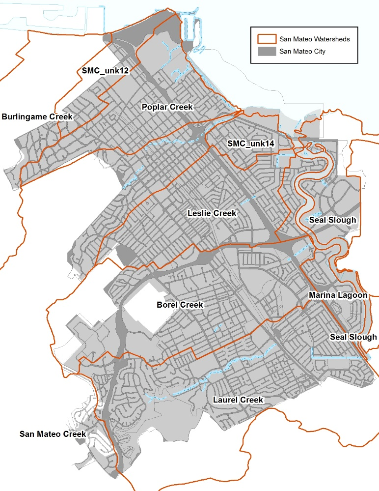
Figure 2-2. Map showing City of San Mateo watersheds and drainage areas included in the demonstration project. Orange lines delineate each watershed boundary. Note that some watershed boundaries are outside the City.
Table 2-1. Regional GIS data layers included in the Site Locator Tool.
|
GIS Data Layer Name |
GIS Data Layer Description |
|
CPAD_2014a2_Holdings |
California Protected Areas database released in the first half of 2014 |
|
FEMA_NFHL |
National Flood Hazard Layers for all BA counties |
|
Employment_Investment_areas_SCS |
From ABAG's data webpage |
|
Priority Development Areas_Current |
From ABAG's data webpage. Priority Development Areas (Current) - This feature set contains changes made to Priority Development Areas since the adoption of Plan Bay Area. DO NOT USE this feature set for mapping or analysis related to Plan Bay Area. |
|
K_12_Schools |
Schools in the bay area (point data) |
|
NLCD2011_PercentImpervious |
Percent Impervious data from the 2011 National Land Cover Dataset |
|
OSM_Buildings |
Open Street Map layer for the Bay Area _Late2014 |
|
OSM_Libraries |
Open Street Map layer for the Bay Area _Late2014 |
|
OSM_Parking |
Open Street Map layer for the Bay Area _Late2014 |
|
OSM_Parks |
Open Street Map layer for the Bay Area _Late2014 |
|
OSM_Schools |
Open Street Map layer for the Bay Area _Late2014 |
|
OSM_Streets |
Open Street Map layer for the Bay Area _Late2014 |
|
R2_CARI_PublicV |
California Aquatic Resource Inventory for Region 2 |
|
Regional_Bike_Facilities_Bay |
Regional bike facilities for the Bay Area |
|
RWQC_RB_2 |
Region 2 Water Board Boundary |
For the city of San Mateo, the primary driver for implementing GI was the Sustainable Streets Plan. Since this plan focused on streetscape redevelopment, spatial data that quantified street and sidewalk attributes and integrated Complete Street concepts were important data for inclusion in the Tool. The City elected to run each of the Tool analyses including the Regional Base Analysis.
Primary locations identified by the City were public parks, pedestrian trails, wide streets, wide sidewalks, existing planters, and parking lots. The city also identified planning opportunities such as areas planned for redevelopment (PDAs), areas of damaged streets/sidewalks, Greenway Networks, and Regional Bike Facilities as well as constraints to GI implementation including sidewalks with large trees, fire lanes, and narrow streets. These opportunities and constraints were then categorized into factors such as funding opportunities, local development opportunities, community visibility, and installation feasibility. These factors were then weighted to produce a relative ranking of areas for potential GI implementation,
The City also included a data layer that identified City-owned parcels in the ownership analysis which allowed for a public/private delineation of locations in the map outputs. The last analysis removes areas that are not feasible GI locations such as wetlands, riparian areas, and areas with utility mains close to the surface. The City excluded all areas intersecting existing wetlands and the San Mateo Lagoon in this analysis. Table 2-2 shows the regional and local GIS data layers included in the Site Locator Tool for the City of San Mateo.
2.5 Site Locator Tool Results
Running the Site Locator Tool with the City of San Mateo was an iterative and interactive process. The first round of conversations with the City focused on identifying street data that had spatial attributes for measuring existing street width. During subsequent conversations, additional data sets such as existing and potential pedestrian trails, sidewalk width, areas of existing sidewalk planters, and regional bike facilities in or identified as additional data that captured certain aspects of the Sustainable Streets Plan. This progression shows how GIS data layers can be added and removed, rankings and data layer weights can be changed. Additionally the Tool can be rerun by including or excluding any of the analyses. This iterative process can be refined as questions and goals change or more accurate local data are available. Based on selected regional and local data layers and the City’s ranking and weighting of these layers, the Site Locator Tool identified 18 acres of City-owned property or right-of-way as highly ranked locations for potential GI implementation, 113 acres as moderately ranked, and 11 acres as lower ranked locations (Figure 2-3). In total, 142 acres were identified as potential locations for Green Infrastructure. Higher ranked sites were the result of relatively higher factor weights on Priority Development Areas and funding opportunity data layers.
Table 2-2. Local and regional GIS data layers included in the Site Locator Tool for the City of San Mateo.
|
GIS Data Layer Name |
GIS Data Layer Description |
Data Layer Type |
Analysis |
|---|---|---|---|
|
Sidestreet parking |
Side Parking polygons on one lane streets (Where Width from Street Saver data* allowed for the minimum dimentions of lanes, medians and parking spaces for each street type and context from the San Mateo Sustainable Streets report) |
Regional/Local |
Locations |
|
Sidestreet parking |
Side Parking polygons on one lane streets (Where There is no Width value from Street Saver data and the minimum dimentions of all street comonants for each street type and context from the San Mateo Sustainable Streets report is assumed) |
Regional/Local |
Locations |
|
Sidestreet parking |
Side Parking polygons on multi lane streets (Where Width from Street Saver data* allowed for the minimum dimentions of lanes, medians and parking spaces for each street type and context from the San Mateo Sustainable Streets report) |
Regional/Local |
Locations |
|
Sidestreet parking |
Side Parking polygons on multi lane streets (Where There is no Width value from Street Saver data and the minimum dimentions of all street comonants for each street type and context from the San Mateo Sustainable Streets report is assumed) |
Regional/Local |
Locations |
|
Sidewalk |
Sidewalk Polygons (Where the width attribute from the San Mateo Sidewalk layer allows for the mimimum dimentions of sidewalk compoents for each street type and context according to the San Mateo Sustainable Streets report and allowed for a GI installation in the sidewalk furniture zone) |
Local |
Locations |
|
Sidewalk |
Sidewalk Polygons (Where there is no width attibute from the San Mateo Sidewalk layer, and minimum dimention of sidewalk compoents from the San Mateo Sustainable Streets report are assumed). |
Local |
Locations |
|
Parking lot |
Parking Facilities quried from San Mateo's facility polygon layer |
Local |
Locations |
|
Pedestrian Trails |
San Mateo's Pedestrian Trail layer buffered 2 ft on both sides (4 ft wide) |
Local |
Locations |
|
Potential Pedestrian Trails |
San Mateo's Potential Pedestrian Trail layer buffered 2 ft on both sides (4 ft wide) |
Local |
Locations |
|
Parking_OSM |
Parking polygons querried from SF Bay OSM polygons (downloaded in August 2014) |
Regional |
Locations |
|
Parks_OSM |
Park polygons querried from SF Bay OSM polygons (downloaded in August 2014) |
Regional |
Locations |
|
CPAD_Areas |
California Protect Areas Database Polygons for the Bay Area |
Regional |
Locations |
|
Sidewalk planter |
Sidewalk Polygons that have a planter width value of 4ft or more |
Local |
Locations |
|
Sidewalk |
Sidewalk Polygons that have a width value of 8ft or more |
Local |
Locations |
|
Priority Development Areas |
Bay Area Wide Priority Development Areas from ABAG |
Regional |
Opportunities and Constraints |
|
Storm Line |
A 25 ft. buffer from the San Mateo Storm Line layer |
Local |
Opportunities and Constraints |
|
Storm Line |
A 50 ft. buffer from the San Mateo Storm Line layer |
Local |
Opportunities and Constraints |
|
Catch basin |
A 25 ft. buffer from the San Mateo Storm Catch Basin Layer |
Local |
Opportunities and Constraints |
|
Street Trees |
A 20 ft. buffer from the San Mateo Urban Tree layer |
Local |
Opportunities and Constraints |
|
large trees ( > 20) |
A 30ft buffer around trees that are over 20ft in circumference from the San Mateo Urban Tree layer |
Local |
Opportunities and Constraints |
|
Street Lights |
A 15ft buffer around street lights from the San Mateo Street Light layer (+5ft for spatial inacuracies between layers) |
Local |
Opportunities and Constraints |
|
Narrow Street_Fire Running Lanes |
A 40 ft. buffer from a selection from the San Mateo Fire Running Lane layer (streets that were less than or equal to 40 ft. wide accounting for spatial inaccuracies in the data layers used) |
Local |
Opportunities and Constraints |
|
Regional Bike Facilities |
A 15 ft. buffer from the Bay Wide Regional Bike Facilities Layer from MTC (+ 25ft to account for spacial inacuracies between layers) |
Regional |
Opportunities and Constraints |
|
Streetside parking |
A Road polygon later create from San Mateo road centerlines buffered half width of that road (Street Saver data* width) taken from the San Mateo location street layer, where the width from Street Saver data* allows for the minimum width of street components for that particular street type and context as well as the minimum width of a bike lane |
Regional/Local |
Opportunities and Constraints |
|
Damaged Streets |
A Road polygon layer (San Mateo road centerline buffered by half of that street's width according to Street Saver data*) where PCI is less than or equal to 40, indicating that they are damaged roads and may need to be repaired soon |
Local |
Opportunities and Constraints |
|
Damaged Sidewalk |
San Mateo Sidewalk polygons that are indicated as having damaged curbs, gutter and or sidewalks |
Local |
Opportunities and Constraints |
|
GreenWay Network |
San Mateo pedestrian priority green way corridor from Ken Chen, Sep 2014 (buffered 85 feet to account for spatial inacuracies and missalignment of layers.) |
Local |
Opportunities and Constraints |
|
Streams |
A 500ft buffer from a subset of San Mateo's Stream layer where no Streams intersect San Mateo's Lake layer |
Local |
Opportunities and Constraints |
|
Lakes |
A 400ft buffer from San Mateo's Lake polygon layer |
Local |
Opportunities and Constraints |
|
Schools |
A 100ft buffer from San Mateo's School polygon layer |
Local |
Opportunities and Constraints |
|
Libraries |
A 100ft buffer from San Mateo's Library polygon layer |
Local |
Opportunities and Constraints |
|
City Hall |
A 100ft buffer from City Hall polygons selected from San Mateo's Facility polygon layer |
Local |
Opportunities and Constraints |
|
parks |
A 100ft buffer from a subset of San Mateo's Facility polygon layer where FACTYPE is = to "PARK" |
Local |
Opportunities and Constraints |
|
City-owned parcels |
San Mateo's city owned parcel layer |
Local |
Ownership |
|
CARI Wetlands |
CARI Wetland polygons: see http://www.sfei.org/it/gis/cari |
Regional |
Knockout |
|
SM_Lagoon |
Lagoon Layer from San Mateo |
Local |
Knockout |
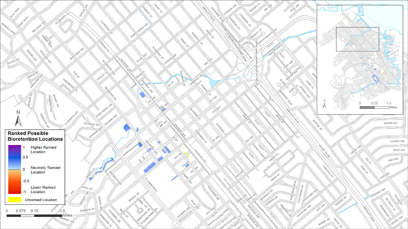
Figure 2-3 Map output of ranked potential bioretention locations in the City of San Mateo. Higher ranked locations are dark blue, lowest ranked locations are red and yellow designates unranked areas due to lacking data in those places
San Mateo and SFEI performed a remote data validation exercise in order to see how the Tool ranked areas previously identified for potential GI implementation. Specifically, Grant Street and Fremont Street were investigated to determine why one street ranked higher than the other. Grant Street was ranked higher than Fremont Street since it had a planned bike lane, which was given a higher weight in the Opportunities and Constraints Analysis. Delaware Street and Bay Meadows were unranked in the output because they were excluded as possible locations due to site characteristics deemed not feasible for implementing GI. Overall, many of the sites identified and ranked highly by the locator tool were also sites that were previously identified as potential GI opportunities by San Mateo. Furthermore, additional high ranked locations were identified which provided the City with additional locations to investigate further and to compare to the current GI plan.
Case Study: San Jose’s Urban Villages
Chapter 3
The city of San Jose is the largest municipality in the Bay area with an area of 180 square miles and a population of over 1 million people (Figure 3-1). Like many cities in the region, San Jose has undergone significant growth over time and experienced environmental issues typically associated with urbanization including increased loadings of sediment, PCBs, mercury, and pathogens. The City is regulated by the Municipal Regional Stormwater NPDES Permit (MRP), and stormwater management is a driver for a number of City activities and area-wide programs.
In compliance with the MRP, the City is currently implementing four green street projects in various stages of construction and design. The City is also continuing to look for opportunities to integrate GI features into existing infrastructure and planning efforts. Envision San Josè 2040, the City’s current General Plan promotes the development of Urban Villages (Figure 3-1) which are active, walkable, bicycle-friendly, transit-oriented, mixed-use urban settings for new housing and job growth attractive to an innovative workforce and consistent with the plan's environmental goals. The urban village strategy fosters: 1) Mixing residential and employment activities; 2) Establishing minimum densities to support transit use, bicycling, and walking; 3) High-quality urban design; and 4) Revitalizing underutilized properties with access to existing infrastructure[1]. Within the development area of the proposed Urban Village, the City is planning to retrofit existing facilities and incorporate new stormwater treatment to address stormwater planning needs, MS4 and TMDL requirements, and local stakeholder concerns.
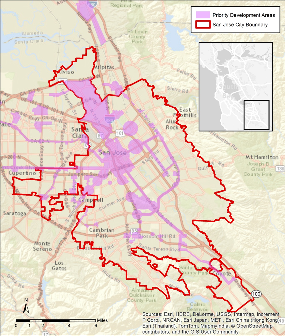
Figure 3-1 City of San Jose and Proposed Urban Villages
3.1 Case Study Objective
To plan for current and future effort to incorporate GI at the City’s landscape, the City needed a planning tool to help determine areas of opportunity and constraint for implementing GI on a wide scale and embraced the GreenPlan-IT Toolkit as a Tool that meets their needs. In discussions with SFEI, the city staff decided to use the redevelopment of the Urban Village as a case study area to test the applicability of the Toolkit. The objective of the pilot study was to demonstrate the capacities and usability of the GreenPlan-IT Toolkit in identifying feasible and cost-effective GI locations at a watershed scale. Results from the Toolkit application will be used to: 1) identify specific green infrastructure projects; 2) support the City’s current and future planning efforts, such as the development of the San Jose Storm Drain Master Plan; and 3) help comply with future Stormwater Permit requirements. At the end of the pilot study, the city staff hoped to have opportunity maps of possible GI locations, a cost-effectiveness curve for flow or pollutant reduction, and a workable Toolkit that can be used for future GI planning efforts.
The downtown area and north San Jose were identified as environmentally and fiscally beneficial locations to develop some of the Urban Villages (Figure 3-1). The majority of this proposed new development is located within the lower part of the Guadalupe River Watershed (Figure 3-2). In consultation with the city staff, the lower part of the Guadalupe watershed was selected for the development of a GreenPlan-IT Toolkit case study. Data are available in this watershed to support the full application of the Toolkit.
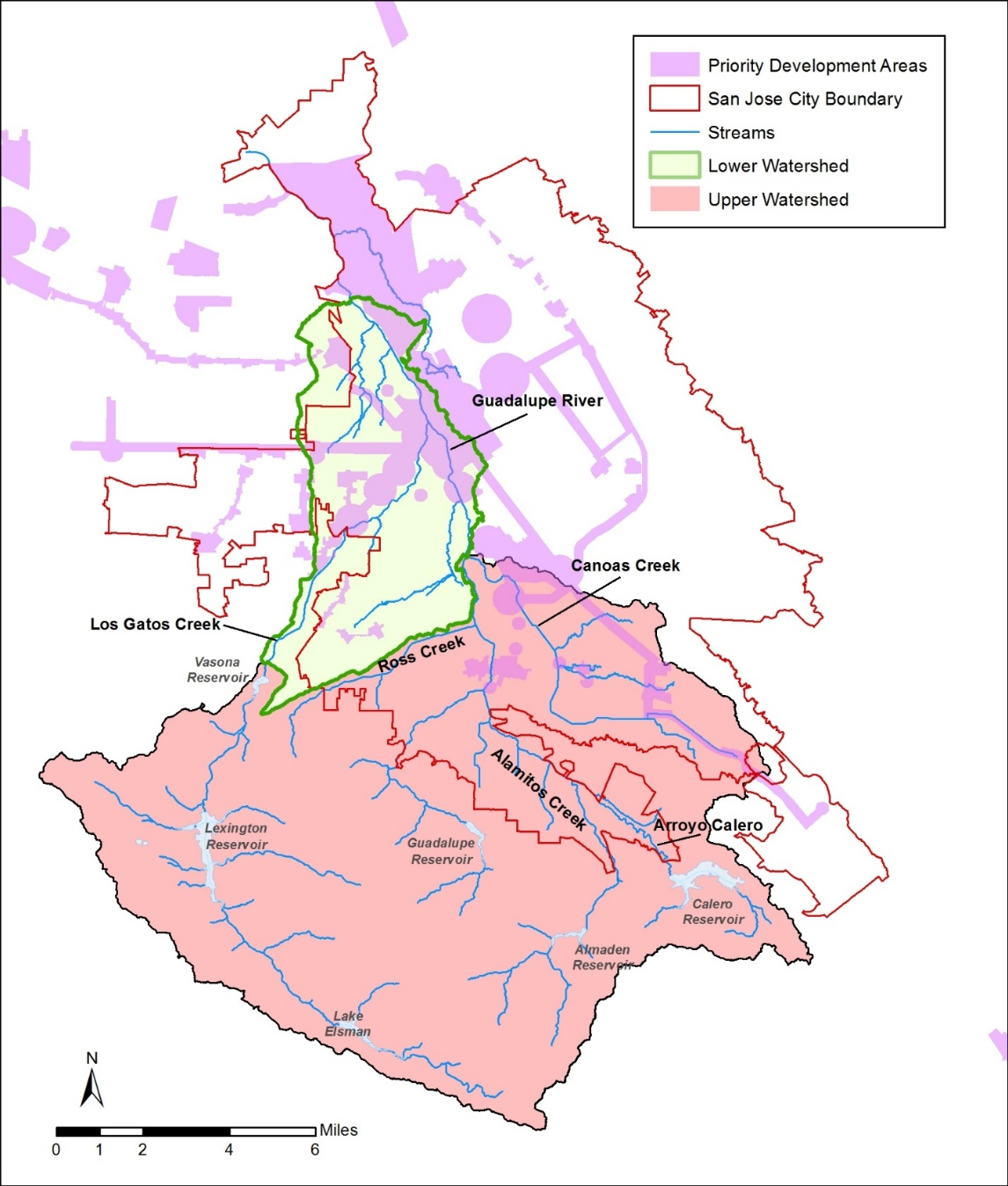
Figure 3-2 Guadalupe River Watershed and Proposed Urban Villages
3.2 Project Setting
The Guadalupe River Watershed is located in the Santa Clara Valley basin and drains to Lower South San Francisco Bay (Figure 3-2). The watershed is the fourth largest in the Bay Area with approximately 170 mi2 of total drainage area. Five main tributaries drain to the Guadalupe River. Six water conservation and storage reservoirs in the watershed provide varying amounts of flood control. The Guadalupe Watershed has a mild Mediterranean-type climate generally characterized by moist, cool wet winters and warm dry summers. Rainfall follows a seasonal pattern with a pronounced wet season that generally begins in October or November and can last to April or May, during which an average of 89% of the annual rainfall occurs (McKee et al., 2003).
The primary focus of this case study is downtown San Jose, and accordingly, the watershed boundary was adjusted to exclude upstream watersheds where gauge data are available to be included as boundary conditions for the appropriate streams and/or sub-watersheds (Figure 3-2). The resulting study area is referred herein as the Lower Guadalupe River watershed with an area of 18,613 acres.
3.3 Site Locator Tool: Data layers used and decision process
The GIS Site Locator Tool integrates regional and local GIS data and uses these data, through an identification, ranking and weighting process, to locate potential GI locations at a watershed scale. Data accuracy is an important determinant in the accuracy of map outputs produced by the Tool. The quality, scale and accuracy of the input data will determine the quality, scale and accuracy of the output maps. Therefore, it is highly beneficial to use more accurate and local data when available. When using more regional scale data layers for analyses, such as the opportunities and constraints ranking analysis, the user can weight and rank these layers to reflect the confidence in local accuracy of the data. There are many regional GIS data that are included in the Tool (Table 3-1) and additional regional data sets can be added as well. Local data sets can be added to the Tool in order to help identify potential locations that meet the goals and planning needs of each city. Each municipality will identify a set of questions or goals to answer or meet prior to running the Tool. These questions or goals become the drivers for deciding which data sets to include.
Table 3-1. Regional GIS data layers included in the Site Locator Tool.
|
GIS Data Layer Name |
GIS Data Layer Description |
|
CPAD_2014a2_Holdings |
California Protected Areas database released in the first half of 2014 |
|
FEMA_NFHL |
National Flood Hazard Layers for all BA counties |
|
Employment_Investment_areas_SCS |
From ABAG's data webpage |
|
Priority Development Areas_Current |
From ABAG's data webpage. Priority Development Areas (Current) - This feature set contains changes made to Priority Development Areas since the adoption of Plan Bay Area. DO NOT USE this feature set for mapping or analysis related to Plan Bay Area. |
|
K_12_Schools |
Schools in the bay area (point data) |
|
NLCD2011_PercentImpervious |
Percent Impervious data from the 2011 National Land Cover Dataset |
|
OSM_Buildings |
Open Street Map layer for the Bay Area _Late2014 |
|
OSM_Libraries |
Open Street Map layer for the Bay Area _Late2014 |
|
OSM_Parking |
Open Street Map layer for the Bay Area _Late2014 |
|
OSM_Parks |
Open Street Map layer for the Bay Area _Late2014 |
|
OSM_Schools |
Open Street Map layer for the Bay Area _Late2014 |
|
OSM_Streets |
Open Street Map layer for the Bay Area _Late2014 |
|
R2_CARI_PublicV |
California Aquatic Resource Inventory for Region 2 |
|
Regional_Bike_Facilities_Bay |
Regional bike facilities for the Bay Area |
|
RWQC_RB_2 |
Region 2 Water Board Boundary |
The primary drivers for GI implementation in the City of San Jose are the redevelopment Urban Villages plan and the Storm Drain Master plan. As noted previously, the Urban Villages plan focuses redevelopment in downtown San Jose for walkability, bikeability, access to public transit, and employment. The Storm Drain Master plan is a large-scale effort to analyze deficiencies in the stormwater drainage network (both storm drain and natural drainage) and provide long-term solutions to the identified deficiencies. The Plan’s goals are to improve water quality, provide flood protection, enhance and protect habitat, and increase stormwater infiltration. Together, these plans provide the pathway for future GI implementation.
San Jose also requested that infiltration trenches be added to the RBA. The Santa Clara Valley has suitable soils for infiltration to groundwater and regional large-scale infiltration trenches are being considered as one mechanism for groundwater recharge. This feature type was added and ranked for each of the five existing metrics (slope, depth to groundwater, soil type, land use, and risk of liquefaction) used for determining suitable locations.
During the first analysis for the City, potential locations were focused on parks, city-owned parcels, wide streets, existing sidewalk planters, and parking lots as potential locations for GI implementation. Formulas were developed, using existing City data, to identify streets and sidewalks with appropriate widths for implementation of bioretention features and parking lots greater than 7000 ft.². The City identified planning opportunities such as areas planned for redevelopment (PDAs), existence of stormwater infrastructure, and planned bikeways as well as constraints to GI implementation including proximity to riparian areas and gas mains. These opportunities and constraints were then categorized into factors (local development opportunities, community needs, conservation, and installation feasibility). These factors were then weighted to produce a relative ranking of areas for potential GI implementation. Community needs and local development opportunities were given the highest weight.
The City also included a data layer that identified City-owned parcels in the ownership analysis which allowed for a public/private delineation of locations in the map outputs (Table 3-2). For the Knockout Analysis, The City excluded all areas intersecting existing wetlands and proximity to other waterbodies (salt ponds, existing percolation ponds, and a 10ft buffer from creek centerlines) as well as existing GI features. The first Tool run included map outputs for bioretention units, permeable pavement, and infiltration trenches. This first run identified approximately 400 acres of moderate to highly ranked areas for potential GI implementation.
After review of the preliminary Tool outputs, city of San Jose staff decided that a second analysis, with modifications made to a few analyses, could help refine their output (Table 3-2). In particular, the City wanted to run the Tool while both including and excluding the Regional Base Analysis (two separate Tool runs). By excluding the RBA, additional locations were included in the analysis and in the map outputs. No new additions were made to the Locations Analysis while there were changes made to the Opportunities and Constraints Analysis. A data layer delineating Urban Villages was added and more heavily weighted in the local development opportunity factor. San Jose’s three-year re-pavement plan was also added and the RBA was added and ranked in lieu of running the RBA at the start of the analysis. Constraints were also removed from this analysis and layer and factor weights recalculated. Installation feasibility (existing storm drain infrastructure) was the highest weighted factor followed by local development opportunities, and community needs (planned bike paths). The City also added additional data to the Knockout Analysis including existing salt ponds and building footprints.
Table 3-2 shows the regional and local GIS data layers included in the Site Locator Tool for the City of San Mateo.
|
GIS Data Layer Name |
GIS Data Layer Description |
Data Layer Type |
Analysis |
|---|---|---|---|
|
Parks |
Layer of city parks |
Local |
Locations |
|
Sidestreet parking |
Data layer identifying streets with on-street parking |
Local |
Locations |
|
Sidewalk planter |
Data layer identifying existing sidewalk planters |
Local |
Locations |
|
Parking lot |
Data layer identifying parking lots with building footprints removed |
Regional |
Locations |
|
City-owned parcels |
Data layer identifying city owned property |
Local |
Locations |
|
Priority Development Areas |
Bay Area Wide Priority Development Areas from ABAG |
Regional |
Opportunities and Constraints |
|
Urban Villages |
Areas within the city of San Jose designated for development of urban villages |
Local |
Opportunities and Constraints |
|
Stormwater infrastructure |
Locations of stormwater mainlines buffered 80 ft |
Local |
Opportunities and Constraints |
|
Stormwater infrastructure |
Locations of stormwater manholes buffered 90 ft |
Local |
Opportunities and Constraints |
|
Stormwater infrastructure |
Locations of inlets to storm drain network buffered 60 ft |
Local |
Opportunities and Constraints |
|
Planned bikeways |
Layer showing all planned bikeways buffered 80 ft |
Local |
Opportunities and Constraints |
|
Repavement plan |
City of San Jose replacement plan buffered half of the street Face of Curb width |
Local |
Opportunities and Constraints |
|
CARI wetlands |
Wetland locations from CARI |
Regional |
Knockout |
|
Building footprint |
San Jose building footprint data layer |
Local |
Knockout |
|
Creek buffer |
Santa Clara Valley Water District 10 ft buffer for existing creeks and riparian areas |
Local |
Knockout |
|
Percolation pond |
Santa Clara Valley Water District percolation ponds data layer |
Local |
Knockout |
|
Various waterbodies |
Other waterbodies for exclusion |
Local |
Knockout |
|
Existing salt ponds |
Santa Clara Valley Water District existing salt ponds data layer |
Local |
Knockout |
|
data\SanJoseDatasets.gdb\OM_Inventory |
Data layer showing locations of existing green infrastructure |
Local |
Knockout |
|
Schools |
San Jose school data layer |
Local |
Knockout |
|
City-owned parcels |
San Jose city-owned parcels |
Local |
|
3.1 Site Locator Tool Results
During the last Tool iteration, City staff requested two Tool runs. The first run included the RBA as designed while the second run added the RBA to the Opportunities and Constraints Analysis where it was ranked and weighted. In the second run, the RBA was not included at the start of the analysis. The first run excluded many possible areas that did not meet the criteria underlying the RBA. For the second run, (including the RBA layers in a later analysis), the relative importance of these criteria can be controlled through the weighting process. City staff found the map outputs from the second analysis more helpful in the process of identifying possible GI locations as it allows for viewing all locations but provides the relative ranks for locating highest opportunity sites. Each iteration of the Tool analysis produced a map with ranked possible locations for bioretention, infiltration trench, and pervious pavement implementation (Figure 3-3). For bioretention, the final map output had a total of 9840 acres ranked from low to high potential. Eighy-five acres were highest ranked (a rank greater than 0.4), while 1705 acres were moderately ranked (a rank between .4 and .2), 3489 acres were ranked relatively low (a rank below .2), and 4559 acres were unranked.
Once the final output was produced, City staff reviewed maps through the lens of the Urban Villages planning efforts as well as other GI planning efforts. One way in which the Tool maps can be helpful is to show alternative locations when particular constraints are identified in planned locations. San Jose was exploring 5th Street and Hedding Street as a potential GI location. This location was ranked relatively lower on the map output due to the street not having an existing storm drain. City staff gave storm drain infrastructure the highest categorical weight in the analysis which resulted in the 5th and Hedding Street area being ranked relatively lower. However during review of the map outputs, a more suitable, and relatively higher ranked, location was identified nearby at 6th and Hedding.
This remote ground truthing is an important step in the process. This can also be combined with a field ground truth effort. The field effort provides real world syntax to how the Tool performed and also identifies other opportunities and constraints that the Tool didn’t capture (due to lacking data or the weighting process). City staff participated in a field ground truthing effort with the Project team. Three locations were visited: Tully Road and 7th Street, Chynoweth Avenue, and the corner of Round Table Drive and Roeder Road. The Tully Road site was identified by the Tool based on a large road median with curbed boundaries. The median is bordered by a busy three lane road, an access turn lane, and a smaller infrequently used one lane road. Discussions at the site centered on drainage patterns to existing storm drains and the potential opportunity to close the one lane road to create a larger GI feature. The Chynoweth site is already in the planning process for bioretention implementation. Site discussions centered on drainage patterns and where bulb outs could be placed. The corner of Round Table Drive and Roeder Road was selected by San Jose Staff as it was a highly ranked location that fell within an Urban Village area. This location was selected in order to demonstrate how the tool could be used to identify locations that had not previously been identified, that also met many of the City’s priorities and criteria for highly suitable locations. Outputs from the Site Locator Tool were then used in the Optimization Tool as described below.

Figure 3.3 Map output of ranked potential bioretention locations in the City of San Jose. Higher ranked locations are dark blue, lowest ranked locations are red and yellow designates unranked areas due to lacking data in those places.
3.6 Modeling Tool
The application of the Modeling Tool involved input data collection, model setup, model calibration, and finally the establishment of a baseline condition.
3.6.1 Data Collection
A large amount of data were collected to support the development of the Modeling Tool.
The input data that were used for developing a SWMM5 model of runoff for Lower Guadalupe River watershed are described below.
- Precipitation Data
The Guadalupe River Watershed is instrumented with numerous meteorological and hydrology stations (Figure 3-4). There are 11 precipitation stations operated by the Santa Clara Valley Water District (SCVWD) and the National Oceanographic and Atmospheric Administration (NOAA). There is a pan evaporation station, which is operated by SCVWD, and an evapotranspiration station, which is operated by California Irrigation Management Information Systems (CIMIS). High-resolution precipitation data (15-minute intervals) were obtained from SCVWD for 3 precipitation gauges-RF1, RF125, and RF-131, located within the Lower Guadalupe watershed (Figure 3-3). The rainfall data from 2010 to 2011 was chosen for model calibration, representing average and dry years. Annual rainfall for each precipitation station is shown in Table 3-3. The precipitation records were analyzed and compared and the Thiessen polygon method was used to assign representative weather stations to sub-basins.
- Evaporation Data
Evaporation is not as spatially or temporally variable as precipitation; hence lower resolution data from more remote sources are adequate for modeling evaporation. Monthly evaporation data for year 2010-2011 at Los Alamitos Recharge Facility in San Jose was obtained from SCVWD (Table 3-4). These data were then converted to monthly average in inches/day as required by the SWMM5 model.
- Land Use Data
The SWMM5 model requires input of land use percentages for each segment to define hydrology and pollutant loads. Land use data was were obtained from the Association of Bay Area Governments (ABAG) 2005 land GIS coverage. The coverage contains 11 different land use classifications, which were than aggregated down to six model categories. The aggregated land use groups for the SWMM5 model and their percentages are listed in Table 3-5.
- Percent of Imperviousness
The percent of imperviousness is an import input data set for SWMM5 hydrology simulation. The GIS layer of imperviousness was from National Land Cover Dataset (NLCD) 2011, which covers the entire lower 48 State at a spatial resolution of 30m pixels (http://www.mrlc.gov/nlcd2011.php). The distribution of impervious land use for Lower Guadalupe watershed is shown in Figure 3-5.
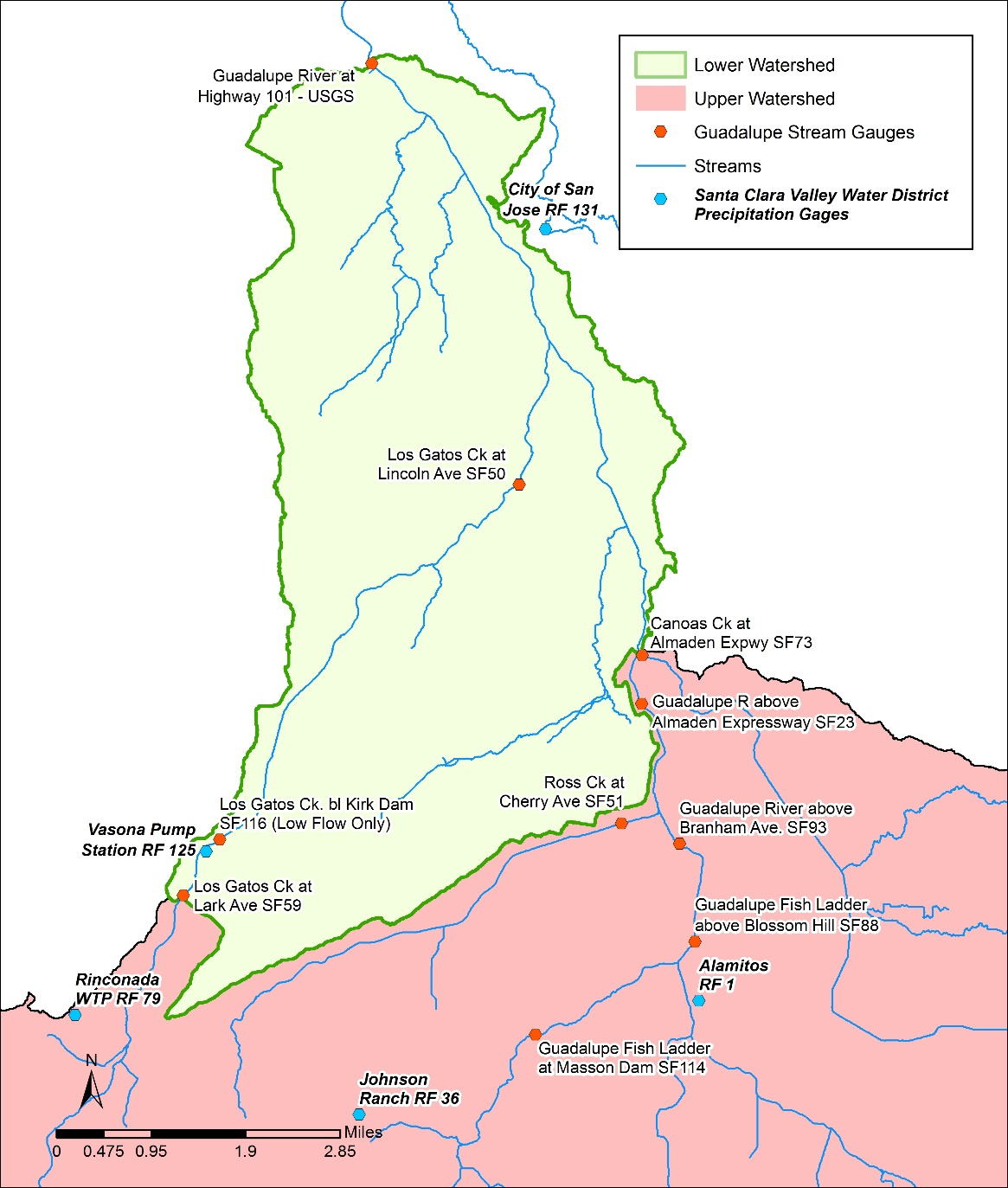
Figure 3-4 Rain gauges and Stream gages in Lower Guadalupe Watershed
Table 3-3 Annual Rainfall (inches) for Precipitation Stations
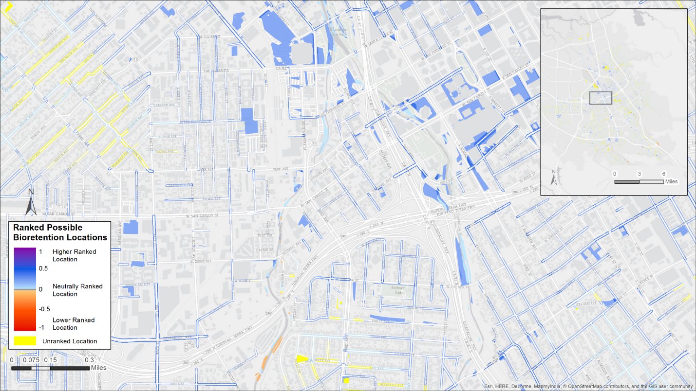
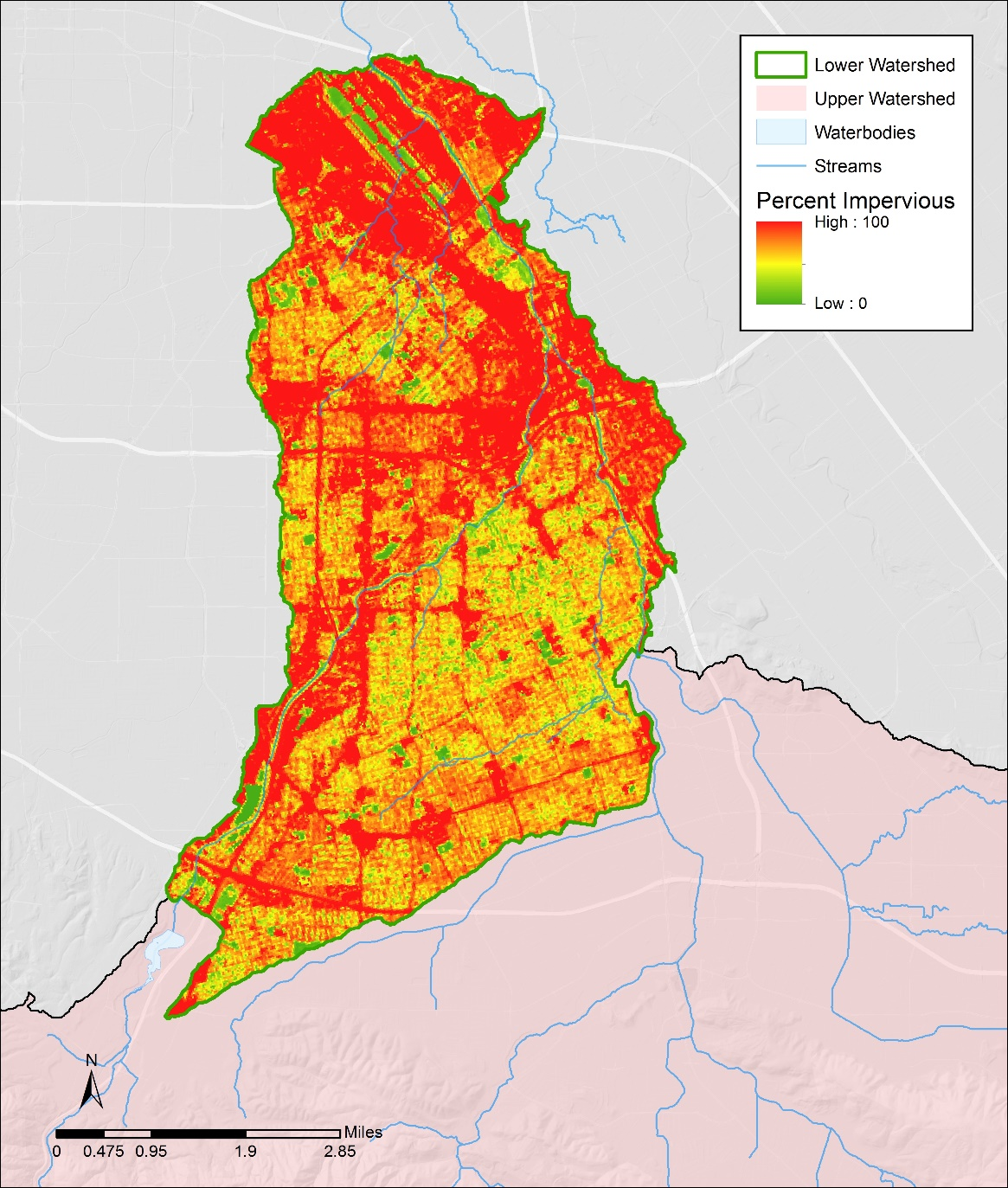
Figure 3-5 Percent of Imperviousness for Lower Guadalupe River Watershed
- Soil Data
Soil data were obtained from the State Soil Geographic Database (STATSGO) and intersected with the subbasin boundary layer to determine the percentages of each soil group for each model segment. STATSGO soils information include the hydrologic soil group (A, B, C, or D) that indicates the ability of the soil to infiltrate water. Soil type can have significant effects on the annual runoff volumes and the peak runoff rates. The Lower Guadalupe River watershed is mainly comprised of D type soils with low infiltration rates and high runoff rates (Figure 3-6).
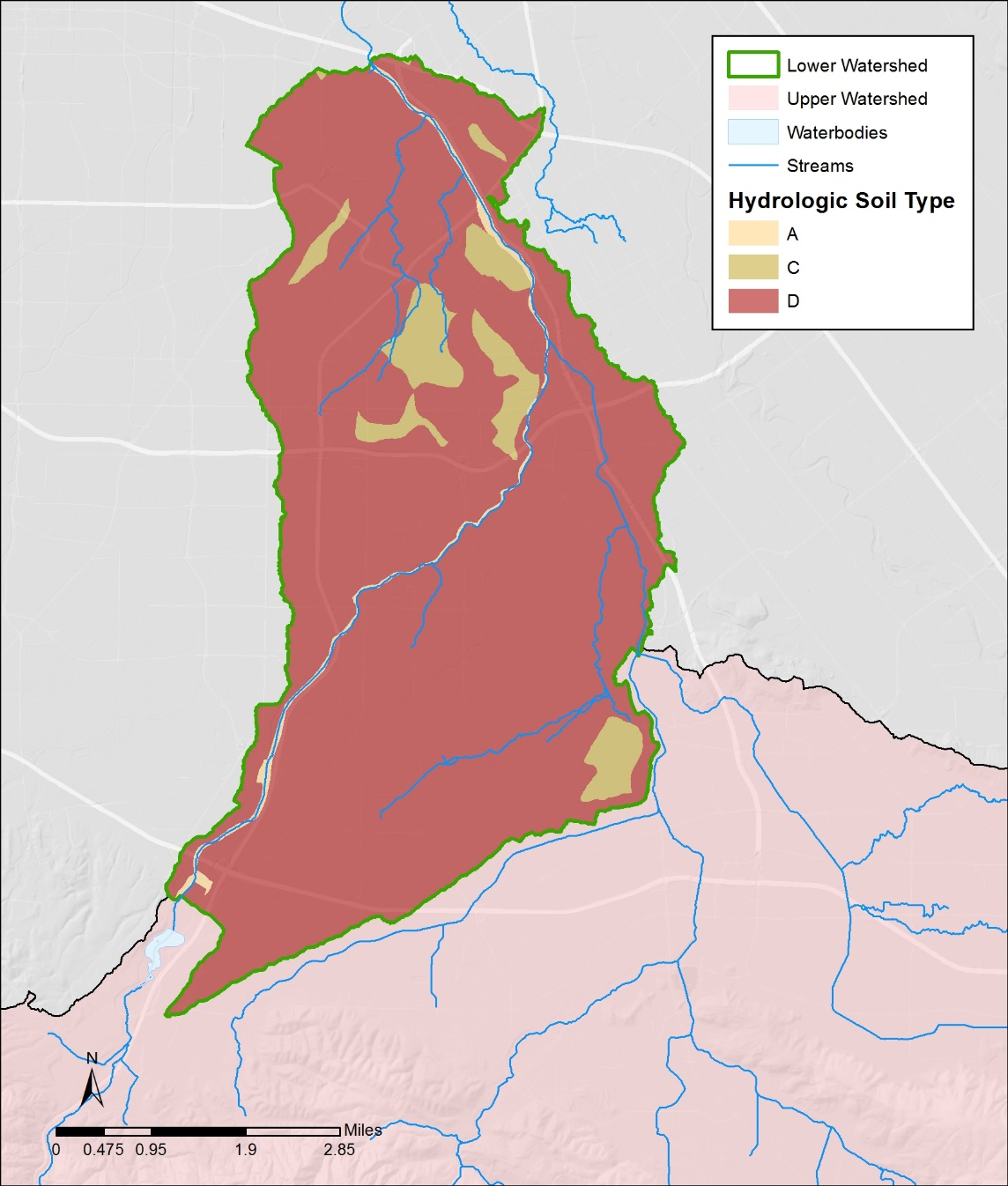
Figure 3-6 Soil Map for Lower Guadalupe River Watershed
- Inflow from Upstream
Flow data for the upstream of the Lower Guadalupe watershed were obtained from three gages at the watershed boundary. Continuous streamflow record (15 minutes interval) from 2010 -2011 was obtained from the SCVWD for stations SF23, SF73, SF59 (Figure 3-4). These data serve as the upstream boundary condition and are input into connected model segments as time series.
- Diversion Data
SCVWD operates a fairly complex water supply system in the Guadalupe River watershed that consists of storage reservoirs, ditches, percolation ponds, and pipelines. Within the modeled area, there are two gauged ditches that divert water from Los Gatos Creek. Daily flow diverted from these ditches was obtained from SCVWD for year 2010-2011. This flow was counted as loss and subtracted from inflow from station SF59.
- Calibration Data
Monitored flow data from 2010 to 2011 at two gages within the model domain were used for model calibration. Daily flow at station SF50 were provided by SCVWD. Flow from the USGS station at highway 101 were downloaded from USGS site http://ca.water.usgs.gov/data/. The USGS station receives water from the entire watershed and is the focal point of model calibration.
3.6.2 Model Setup
The first step in setting up the Modeling Tool is to delineate the watershed into smaller, sub-basins (model segments) using topographical data; the model treats each sub-basin as a homogeneous unit. Through a terrain analysis ArcGIS extension called TauDEM, the Lower Guadalupe River watershed was delineated into 150 sub-watersheds, ranging from 11 to 381 acres (Figure 3-7). Model setup also involves land use reclassification, reformatting input data into SWMM5 model formats, assigning the model segments to proper rain gauge, selecting assessment points, and estimating initial model parameters through GIS analysis and literature review. The time step of model simulation was set as 15 minutes, to be consistent with the resolution of precipitation. The model configuration established a representation of Lower Guadalupe River watershed, and model calibration was then followed to ensure the model parameters reasonably represent the watershed condition.
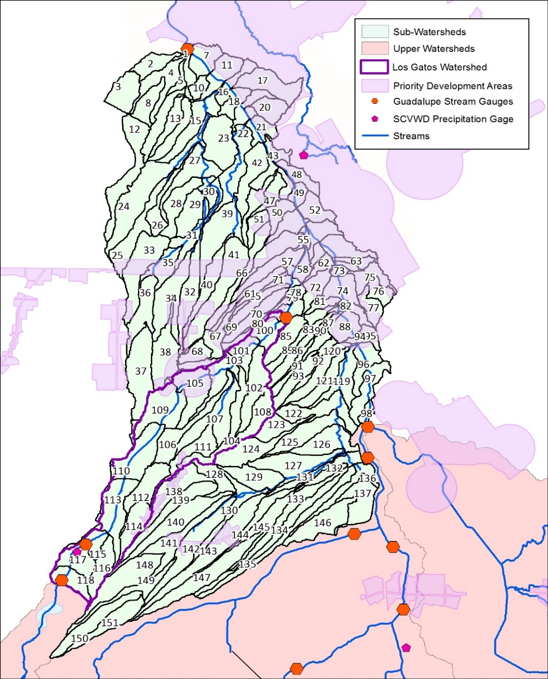
Figure 3-7 Delineated Lower Guadalupe River Watershed
3.6.3 Model Calibration
Model calibration is an iterative process of adjusting key model parameters to match model predictions with observed data for a given set of local conditions. Through the model calibration, it is hoped that the resulting model will accurately represent important aspects of the actual system. The model calibration is necessary to ensure that a representative baseline condition is established with a high degree of confidence in its applicability to form the basis for comparative assessment of various management scenarios.
The hydrologic calibration was performed at two stations (Figure 3-6) within Lower Guadalupe River watershed by means of an iterative process of trial and error using logical adjustments of parameters in consultation with local experts and technical advisors. The calibration started at the tributary station SF50 (Los Gatos at Lincoln avenue) to ensure a reasonable estimates of flow from this tributary. After the calibration was completed at this station, the calibration was then performed at the USGS station at Highway 101, near the mouth of the Guadalupe River. The calibration period was from year 2010 to 2011.
- Baseflow
SWMM5 was originally designed to simulate urban wet weather runoff but does include a method of estimating base flow (dry weather flow) (Rassman, 2010). The baseflow for the Lower Guadalupe River was determined from the measured dry weather flow in 2010 and 2011. A constant flow of 5 cfs was added to two nodes in the tributary and produced an appropriate calibration for the USGS gage.
- Calibration Parameters
SWMM5 is associated with a large number of spatially variable parameters that describe the characteristics of individual subbasins. A subset of the model parameters associated with frequent storm events - impervious percentage, subcatchment width, Manning’s roughness, depression storage, and soil infiltration parameters, are sensitive and typically used as hydrologic calibration parameters. The calibration effort was focused on adjusting these parameters until modeled flow rates match the timing, magnitude, and total volume of the observed data.
The percentage of imperviousness turned out to be the most sensitive parameter, strongly influencing both the total volume of runoff and the peak flows. To obtain a good adjustment of the hydrograph, the initial percentage of imperviousness was decreased 10% for each subcatchment. The subcatchment width is an abstract basin parameter computed by dividing the subcatchment area by the travel length. Because of its inherent uncertainty, this parameter was also used as a major tuning parameter. The travel length was increased for all basins (ranging from 50% to 100%) to create a more attenuated response to storm events. These are reasonable adjustment when taking into account the error margin that can be obtained when estimating these parameters (Wickham, et al, 2013). The parameters of depression storage, infiltration and roughness are less impactful and were adjusted within the range of the established values in the literature to help further improve model calibration.
- Hydrologic Calibration Results
The results of the final calibration are provided in Figure 3-8 and Figure 3-9. At both stations, modeled daily flow match the volume and timing of observed data well, but the peaks of biggest storms were consistently over simulated. Several factors could contribute to this. The inflow from the upstream stations makes up the majority of flow in Guadalupe River and heavily impact the calibration at downstream stations (Figure 3-5). The high flow from these stations were extrapolated from flow-stage curves that often are not calibrated or updated with field measurements during the biggest storms due to lack of personnel and sometimes hazardous conditions (SCVWD, personal communication, 2014). As a result, these flow numbers may not be very reliable and could be biased high. The model uses precipitation data from three rain gages and assigns representative stations to sub-basins based on Thiessen polygon method (Figure 3-4). Localized rainfall events, typical in the Guadalupe watershed as characterized by large variation in mean annual precipitation ranging from 48 inches in the headwaters to 14 inches at the Central San Jose, may not be captured and could contribute to the discrepancy between modeled and observed peak flows. In addition, uncertainty in some key input data such as the percent of imperviousness, local soil conditions, and directly connected impervious area could also introduce uncertainty into the model calibration.
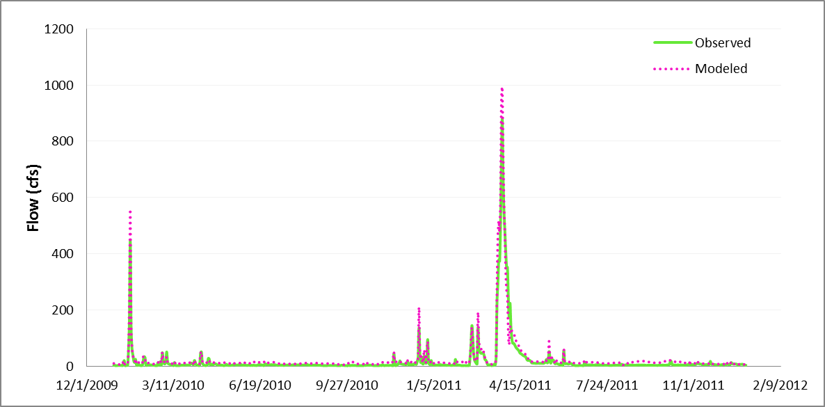
Figure 3-8. Modeled and observed daily flow at Los Gatos Creek, Lincoln Avenue
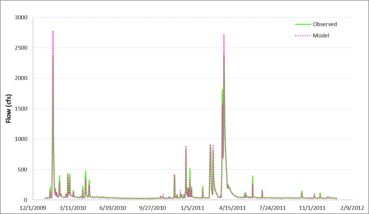
Figure 3-9. Modeled and observed daily flow at USGS station near highway 101
These caveats accepted, the accuracy of the model calibration was also quantified based on the calculated mean error for the modeled and observed storm volume and Nash–Sutcliffe model efficiency (Nash and Sutcliffe, 1970). Both statistics are well within acceptable criteria, indicating an overall good hydrologic calibration; a first indication that the model calibration is quite sufficient to support the GI application.
Table 3-6. Statistics for evaluation model calibration
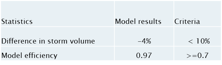
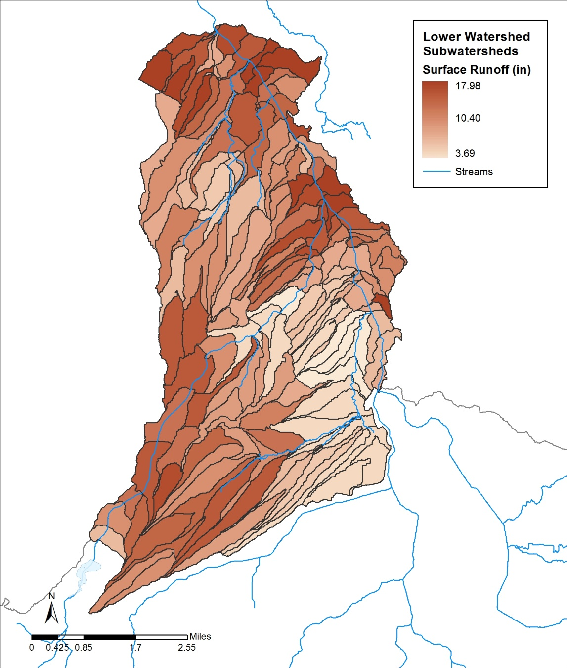
Figure 3-11. Surface Runoff Distribution for Baseline Condition
3.7 Optimization Tool
As the last tool in the Toolkit application, the Optimization Tool repeatedly runs the Modeling Tool to iteratively arrive at the optimized GI scenario. The objective of the Optimization Tool is to determine GI locations, types, and design configurations that minimize the total cost of management while satisfying water quality and quantity constraints. Currently, three GI feature types - bioretention, infiltration trench, and permeable pavement were built in the Tool, as recommended by the project Technical Advisory Committee (TAC). The major steps of this application includes formulating optimization problem, selecting critical storm, designing GI representation, and assigning GI cost.
3.7.1 Focus Area
Downtown San Jose, a primary focus area for redevelopment, was selected from the Lower Guadalupe watershed to demonstrate the application of the Optimization Tool. The selected watershed covers 53 model segments with a total area of 4300 acres (Figure 3-12). The Optimization Tool was to identify cost-effective GI combinations and distributions for the selected area, for which future GI retrofit and implementation are planned to offset the impact of the new development.
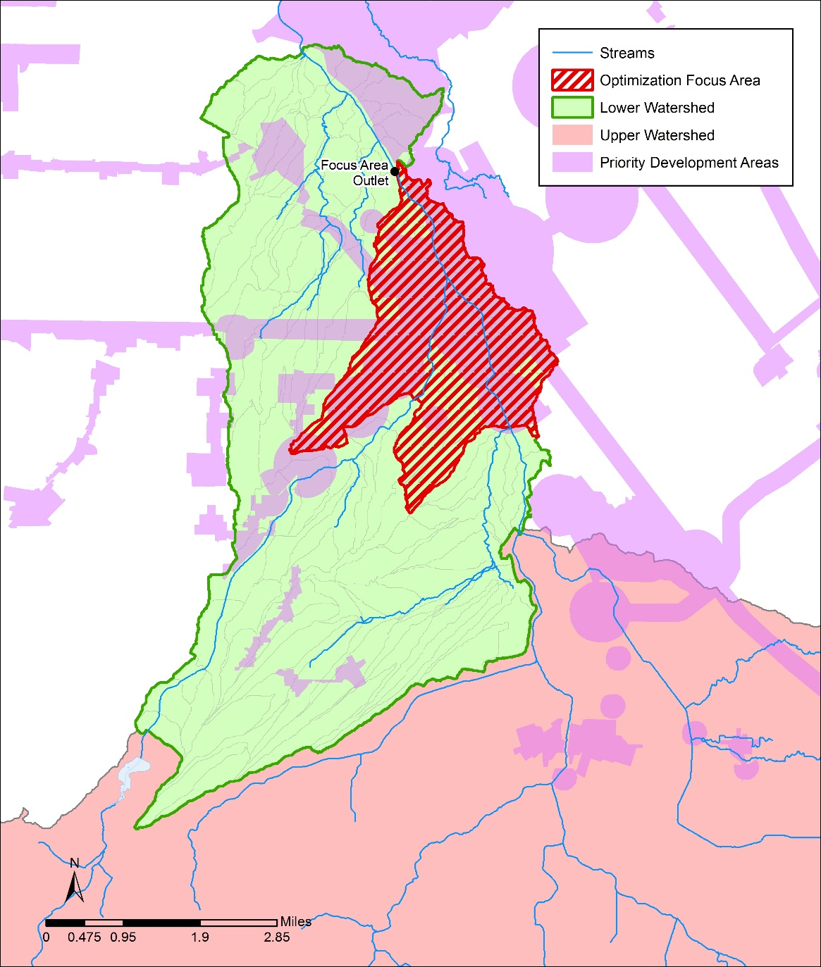
Figure 3-12. Optimization Focus Area
3.7.2 Optimization Problem Formulation
The application of the Optimization Tool began with the formulation of optimization problem, which requires the determination of management targets and selection of assessment point and decision variables.
- Management targets
The determination of management targets is the first step in formulating an optimization problem. These management targets can be based on flow and/or water quality. For example, a management target for flow can be a desired reduction in average annual volume, peak discharge, or exceedance frequency. For this case study, no specific reduction targets were defined, and the overall management targets are to reduce total runoff volume for a design storm event. Therefore, a full range of control targets from 0 -100% were explored, and the optimization was to identify optimal solutions for any possible targets within the range.
- Assessment point
An assessment point is the location in the study basin where runoff or pollutant loading reduction will be evaluated relative to optimization goals. The assessment point for this study is the outlet of the study area (Figure 3-12).
- Decision variables
To run the optimization analysis, the user must define decision variables that will be used to explore the various possible GI configurations. For this analysis, the decision variables are defined as the number of fixed-size units of the distributed GI types. In the Lower Guadalupe San Jose case study, the total number of decision variables ended up as 159 (53 basins*3 GI types). For each applicable GI type, the decision variable values range from zero to a maximum number of potential sites, which were identified by the GIS Site Locator Tool. The decision variables were also constrained by the total area that can be treated by GI within each sub-basin. Through the discussion with the project Technical Advisory Committee (TAC), a 4% “rule of thumb” (defined as GI design at four-percent of the project area to capture 100% stormwater volume of a design storm) was used to size GI for this study. During the optimization process, the combined numbers of GI were forced to be less or equal to the maximum numbers calculated by applying this 4% rule.
3.7.3 Design Storm
The setup of the Optimization Tool also required the selection of a typical precipitation year for use in comparing alternatives and assessing downstream impacts. At the recommendation of the City of San Jose, a 2-year storm with 24-hour duration was selected to drive the simulation process. The storm has a total rainfall of 1.86 inches, according to Santa Clara County’s drainage manual (Santa Clara County, 2007). The distribution of the storm was derived from a normalized rainfall pattern recommended by the manual for use in the San Jose area (Figure 3-13). To be consistent with the resolution of the storm event, the time step in the Modeling Tool as used by the optimization engine was also set at 5 minutes, different from the 15-minute time steps used in the model calibration.
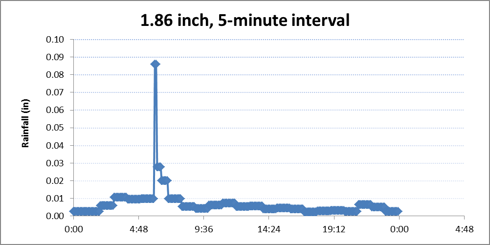
Figure 3-13. Distribution of San Jose 2-year Storm Event with 24-hour Duration
3.7.4 GI Representation
Three GI types - bioretention, infiltration trench, and permeable pavement were included for optimization. Each GI type was assigned a typical size and design configuration that remained unchanged during the optimization process. The decision variables were the number of each GI type within each sub-basin and changing in size of GIs was implicitly reflected through the change of number of GIs implemented. Table 3-5 summarizes key design parameters for each GI feature.
Table 3-6 GI configurations used in Optimization Tool
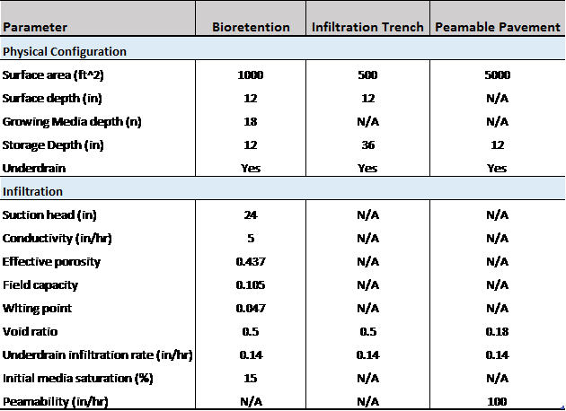
3.7.5 GI Cost
Local sources were used to derive capital cost data for GI on public rights of way. The reliable cost information for each GI feature is critical for identifying optimal solutions, because the optimization process and solutions are highly sensitive to the cost function. A unit cost approach was used to calculate the total cost associated with each GI scenario formed in the optimization process, in which cost per square feet of surface area was specified for each GI type and the total cost of any GI scenario was calculated as:
Total cost = ? (number of each LID type * unit cost * surface area of each LID type)
Implementing GI at the landscape scale would incur many costs ranging from traffic control, construction, to maintenance and operation. For this project, the costs considered were construction, design and engineering, and maintenance and operation (with 20 year lifecycle).
GI cost information for various GI types were collected from literature review, contacting local stormwater agencies, as well as reviewing similar studies in other regions. In general, only limited cost information was available, and these costs vary greatly from site to site due to varying characteristics, different design/configuration, and other local conditions/constrains (Table 3-7). After consulting with the TAC and stakeholders, the cost for bioretention was estimated as $104/square foot (sf) surface area, infiltration trench as $90/sf surface area, and permeable pavement $34/ sf surface area. These cost estimates were used to form the cost function in the Optimization Tool, which were evaluated through the optimization process at each iteration.
Table 3-7 GI unit costs from different sources
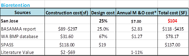
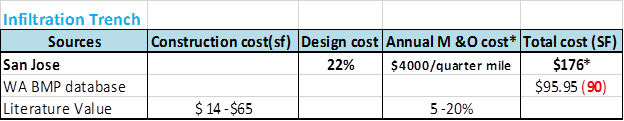
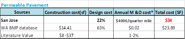
3.7.6 Optimization Results
Consistent with Site Locator Tool analysis, two scenarios were run with the Optimization Tool: with base analysis and without base analysis. With each scenario, the optimization procedure was run for 200 iterations, each with 100 solutions. After which, the optimization converged to final optimal solutions and the process was stopped. The entire process took about 2 hours of computer time from start to finish – a run time deemed reasonable by the TAC; a good tradeoff between spatial resolution and model usability.
- Cost-effectiveness curve
The optimization process outputs the optimal solutions along a cost-effectiveness curve. The curve relates the levels of runoff removal efficiency to various combinations of GI throughout the watershed and their associated cost. Figure 3-14 and Figure 3-15 show the cost-effectiveness curve for scenario with/without base analysis, respectively. For each scenario, all 20,000 individual solutions are plotted together, with the optimum solutions that form the left- and upper-most boundaries of the search domain highlighted in red. Each point on the graph represents one combination of the number of bioretention units, Infiltration Trench, and permeable pavement for each subarea within the study area.
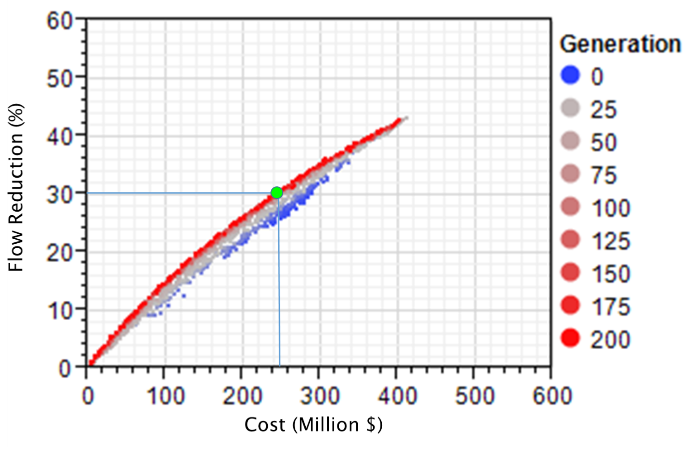
Figure 3-14. Cost-Effectiveness Curve for Scenario with Base Analysis
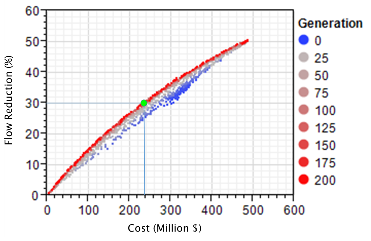
Figure 3-15. Cost-Effectiveness Curve for Scenario without Base Analysis
The cost-effectiveness curve suggests that there exists a largely linear relationship between level of implementation (represented as total cost) and runoff volume reduction, and the maximum achievable runoff volume reduction at the outlet of study area, given the objectives and constraints associated with the study, is approximately 43 percent for with base analysis (Figure 3-13) and 50 percent for without base analysis (Figure 3-14). With the help of this information, decision makers can set realistic goals on how much can be achieved and the level of investment required, as well as determine at what point further investment on GI will yield no improvement on runoff reduction. Between the two scenarios, more GIs (and thus higher cost) will be required for the with base analysis to achieve the same level of runoff reduction (i.e. 30% reduction), as the base analysis excluded some potential sites for more efficient GI types bioretention and infiltration trench, and the optimization was forced to pick more of less efficient types (incurring more cost) to make up the difference. While the cost distribution does not provide specific information about the spatial locations of actual GI features nor the actual cost of build out, knowing the types of practices associated with each point along the cost-effectiveness curve provides insight into the reasoning and order of selecting individual practices.
Of the two scenarios, the City is primarily interested in the scenario without base analysis. Therefore, the discussion of optimization results from here on was focused on this one only.
- Example scenario – 30% reduction
The optimal combinations of GI types and numbers for user-defined reduction goals along the cost-effective curve can be specified. Take the example of a 30% runoff reduction goal, the optimal combination of GI types identified through the optimization process is listed in table 3-8. In total, 3300 GIs will be needed to treat the 4300 acre focus area with a price tag of $240 million based on the model assumptions of GI design and unit cost. The number of each GI type needed for achieving certain reduction goal is generally determined by the collective factors of GI design, cost and potential feasible locations. The actual cost would be much less than the $220 M price tag given the opportunity to reduce unit costs through standardized designs batched implementation, implementation with other road related or drainage related projects, public-private partnerships, reduced need to upsize existing grey infrastructure, and many other benefits not accounted for such as increased property values, reduced heat and other benefits.
Table 3-8 The Number of GI identified for 30% Runoff Reduction

Figure 3-18 Optimal Permeable Pavement Sites for 30% Runoff Reduction
It is important to emphasize that users must interpret the optimization results in the context of specific problem formulation, assumptions, constrains, and optimization goals unique to this case study. If one or more assumptions are changed, for example, the optimization target was designed as reducing peak flow instead of total volume, the optimization might have resulted in a completely different set of solutions in terms of GI selection, distribution, and cost. It also should be noted that because of the large variation and uncertainty associated with unit GI cost information, the total cost associated with various reduction goals calculated form the unit cost do not necessarily represent the true cost of an optimum solution for the basin evaluated and are not transferable to other basins. Rather, these cost should be interpreted as a common basis to evaluate and compare the relative performance of different GI scenarios. The Optimization Tool provides a framework to identify optimal solutions for addressing stormwater management issues at the watershed level.
- Comparison with Results from Site Locator Tool
For the study area, the preliminary GIS screening through the Site Locator Tool identified 23,600 potential sites for GI implementation. These sites could serve as a starting point for GI planning and form the basis for the application of the Optimization Tool. Through the optimization process, not only were the number of sites reduced down to 3300, but the optimal combinations of GI were also identified. (Figure 3 -16). More importantly, the use of the Optimization Tool can provide users with critically needed quantification on cost and benefit (reduction) associated with various management options to help them in finding informed and optimal solutions. Therefore, the application of the full Toolkit is always preferred when sufficient data are available to support the development of the Modeling and Optimization Tools.
3.7.7 Sensitivity Analysis
Previous studies (USEPA 2011, State of Washington 2013) suggested that the optimal process and solutions are highly sensitive to GI cost. A sensitivity test was run to test sensitivity of optimal solutions to GI unit cost estimates. The unit cost for each GI type was changed (Table 3-9), and the optimization procedure was similarly run for 200 iterations with a population size of 100.
Table 3-9 GI unit cost for sensitivity analysis
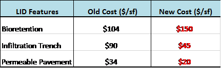
As expected, the sensitivity results suggest that assumptions made with GI cost were highly influential on the optimization modeling results. Varying the unit cost, at the same level of reduction results in different price tags and GI combinations or vice versa (Figure 3-19). For instance, at the 30% runoff reduction level, the total price tag will be $220 million with the original unit cost, but $200 million with the new cost. And the optimal combinations of GI types and numbers are also different. Therefore, reliable and accurate local cost information should be used to drive the optimization process, wherever possible.
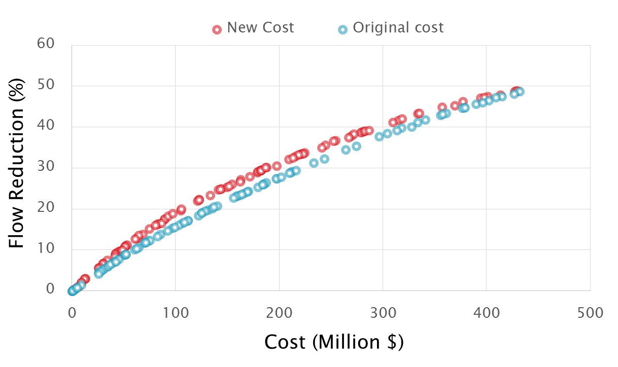
Figure 3-19. Optimal Fronts of Sensitivity Tests
Discussion and Recommendations
Chapter 4
The GreenPlan-IT Toolkit is a planning level tool that provides users with the ability to evaluate the cost effectiveness of GI for addressing stormwater management in urban watersheds. The case study in City of San Mateo demonstrated how the GIS Site Locator tool was used to screen potential sites for GI implementation, while case study in San Jose PDA highlighted the power and utility of the Toolkit and demonstrated how to use the Toolkit to support a cost-benefit evaluation of stormwater runoff control. The two case studies provide useful and practical information that can help managers to understand and evaluate the benefits of GI in urban watersheds.
As illustrated by the San Jose case study, the application of the Toolkit requires careful formulation of the management questions and the optimization objectives. Setting up the Modeling Tool requires deciding on the appropriate spatial scale such as the number of sub-catchments and resolution used to represent GI, as well as the input data collection, model calibration, and development of the baseline condition. The Optimization Tool can be very powerful when combined with hydrologic modeling and cost analysis. Successful and meaningful application of the Optimization Tool largely depends on accurate representation of the watershed baseline condition, GI configurations, and the associated GI costs. The sensitivity analysis demonstrated that the optimization process is highly sensitive to GI cost data used in selecting solutions, and as a result, sensitivity analysis and evaluation of cost control measures or economies of scale are recommended wherever the Toolkit is applied. This section discusses the lessons learned from these case studies, identifies major data gaps, and makes recommendation on future enhancements.
4.1 Lessons learned
The case studies presented in this report provide useful and practical guidance for conducting similar studies in other watersheds. The lessons learned from these case studies could benefit potential GreenPlan-IT users.
- Determination of Spatial Scale
The first challenge in any modeling study is to determine how detailed the model needs to be in order to properly represent the system. The model should only be as complex as necessary to address modeling objectives and answer the management questions. In the context of optimization for GI placement, the study area should be delineated into sub-basins that are small enough to be meaningful for guiding GI implementation while not adding extra burden on model run time. There will always be a trade-off between model spatial resolution and run time. Different choices might be made by first time users versus seasoned users.
- Importance of Model Calibration
The model baseline is the foundation upon which all subsequent analyses depend and is crucial for meaningful results. The importance of a representative baseline model highlights the importance of model calibration. In the San Jose case study, a significant amount of effort was invested to calibrate SWMM using a weight-of-evidence approach to ensure the baseline model adequately represents the existing watershed conditions. Future users of the Toolkit should always bear this in mind and invest effort in model calibration with local data to ensure the meaningful application of the Toolkit.
- Interpretation of Optimization Results
The Optimization Tool performs iterative searches to identify cost-effective solutions. The search process is dependent on the problem formulation, model assumptions, GI cost and GI treatment effectiveness. Therefore, the cost-effective solutions from the optimization process would very much depend on the user-defined goals and assumptions and must be interpreted within the context that defines each specific application. The application of GreenPlan-IT Toolkit must also be accompanied by an intimate understanding of the study area and all influential factors that affect local stormwater management in order to ensure meaningful interpretation of optimization outcomes.
- Consideration of Optimization Run-time
The total number of iterative runs needed for the optimization process to converge to the optimal solutions is dependent on the number of decision variables, model simulation period, and the complexity of the model (number of sub-basins and stream neatwork). More model runs usually leads to longer computation time. For the San Jose case study, it took about two hours for the optimization process to reach optimal solutions after 200 runs, and this short computation time is largely benefited from a very short simulation period (24 hours). If the Optimization Tool is applied to a large watershed with many feasible GI sites and a complex stream network and the optimization process is based on long-term continuous simulation, a large amount of computation time will be needed to reach the optimal solutions. In general, the computational efficiency can be achieved through reducing the number of decision variables, simulation time, and complexity of the problem.
4.2 Data Gaps
The GreenPlan-IT Toolkit is a data-driven tool whose performance is dependent on the availability and quality of the data that support it. Through the two case studies, major data gaps for each tool were identified.
- GIS data
The placement opportunities for GI define the extent to which GI can beneficially impact flow volume. In each of the case study, limitations were placed on the locations available for GI placement, which in turn led to a definition of the maximum potential effectiveness of the GI in controlling runoff volume. Some of these limitations were physical constraints of the landscape that were derived during the engineering and design process. Other limitations were defined based on land use or ownership criteria resulting from the local decision making process. The restrictions placed on GI must be understood in order to evaluate the management scenarios.
- Monitoring data
Developing the Modeling Tool to establish a representative baseline requires the calibration of the model with monitoring data. For the San Jose case study, there were good precipitation time series, long-term flow monitoring data at a number of gages, and good spatial data to characterize land use and impervious cover to support model development. While in the San Mateo case study, lack of monitoring data limited the full utilization of the Toolkit. Lack of monitoring data, in particular water quality data, and general quality issues associated with model input data will be a major hurdle when applying the Toolkit to other watersheds in the Bay Area.
- GI cost information
As demonstrated by the sensitivity analysis of the San Jose case study, the optimization strongly depended on the available GI cost information, and uncertainties in local cost data can greatly influence the management conclusions. GI cost could vary widely from one location to another, influenced by site-specific factors such as physical characteristics, constrains, and local economy. For the San Jose case study, there was very limited information available on GI cost, most of which was for bioretention and little for infiltration trench or permeable pavement. The understanding and utilization of the optimization results must take this limitation into account. To ensure a meaningful application of the Toolkit, reliable local cost information must be collected to drive the optimization process. While it is important to have accurate cost information for each GI type, it is the relative cost difference between GI types that determines what constitutes the optimal GI types and combinations. Therefore, it is crucial to have reliable estimates on relative cost difference between various GI types and interpret the price tags associated with each GI scenario as the relative merits of one scenario verse another, not as the true cost of implementation.
4.3 Future Steps/Enhancements
The case studies showcased in this report were focused on stormwater volume control and represent the first phase of the GreenPlan-IT Toolkit development. To develop a tool that is comprehensive and flexible enough to handle a variety of situations and address a wide range of management questions, the Toolkit needs to be continuously evolving. Future enhancements on the Toolkit are identified through experiences and insights gained from the Toolkit development, case studies, and discussion with the TAC and stakeholders.
- Site Locator Tool
During the next development stage, more GI types could be included in order to develop a wide range of management alternatives. In addition to new GI types, some cities may also be interested in keeping centralized regional facilities such as enlarged bioretention as an option to supplement GI implementation. A diverse set of management options should be evaluated through the Toolkit to provide solutions to a wide range of stormwater management problems. Such additional features could then be considered within the modeling and optimization tool components thus keeping the tool flexible enough to address multiple endpoints such as drinking water supply augmentation or storm sewer master planning. Furthermore, changes to the Site Locator Tool’s Opportunities and Constraints ranking functionality would allow for final ranked locations to contain information showing the reasons it was ranked high or low. Additional work could be done to allow for final outputs to be exported automatically to PDF formats as well as improving current KMZ/ Google Earth format functionality. Moreover, guidance and/or models could be developed to help municipalities create potential location layers needed in the Location Analysis of the Site Locator Tool.
- Water quality simulation/optimization
Currently, SWMM5 lacks mechanisms to simulate water quality reduction through GI implementation. This deficit is the reason why water quality simulation/optimization was not performed for the San Jose case study. Developing methodology and corresponding modules to quantify the pollutant removal efficacy for various GI types will be the first major task for future enhancements. EPA’s SUSTAIN modeling system includes a BMP module that uses a first-order decay approach to estimate the GI performance on pollutant removal. Incorporating this first-order method or use the module directly can be one way to tackle the water quality problems.
- Flexibility in Optimization Tool
The current setup of the Optimization Tool is tailored to the setting of the San Jose case study to expedite the tool development. Many important decision variables such as the total number of iterative runs and the size of the population were predetermined and coded in the tool programs. Next phase of the tool development should make key decision variables of an optimization problem as user-defined inputs to provide flexibility for broad applicability. Having users define these variables will also help them better understand how the tool functions.
- Improved cost function.
A major weakness in the current cost information is associated with cost data being derived from pilot scale one-off implementations. Future improvements of the cost function could include reasonable project batching scales (3- and 4-way intersections redevelopments that include multiple GI features, blocks or multi-block scale redevelopments, neighborhood scale redevelopments, and combinations of GI feature types (e.g. perviois pavement in concert with small and large bioretention)).
- Additional case studies of different settings
The Toolkit was applied to two case studies to demonstrate its power and utility. Additional applications of the Toolkit at other watershed settings will not only provide much needed insights on what the region needs, but also in the process will help improve/refine the Toolkit functionalities to meet these needs.
References
Chapter 5
Deb, K., Pratap, A., Agarwal, S., and Meyarivan, T. (2002). A fast and elitist multiobjective genetic algorithm: NSGA-II, IEEE Transactions on Evolutionary Computation, 6(2) (2002) 182-197.
McKee, L., Leatherbarrow, J., Pearce, S., and Davis, J. (2003). A review of urban runoff processes in the Bay Area: Existing knowledge, conceptual models, and monitoring recommendations. A report prepared for the Sources, Pathways and Loading Workgroup of the Regional Monitoring Program for Trace Substances. SFEI Contribution 66. San Francisco Estuary Institute, Oakland, Ca.
Nash, J.E., and Sutcliffe, J.V. (1970). River flow forecasting through conceptual models part I—A discussion of principles. Journal of Hydrology 10(3):282–290.
Rossman, L. A (2010). Storm Water Management Model User’s Manual, Version 5.0, U.S. Environmental Protection Agency. Office of Research and Development. EPA/600/R-05/040.
Santa Clara County, California, Drainage Manual. Adopted August 14, 2007
State of Washington (2013). Case study for applying SUSTAIN to a small watershed in the Puget Lowland. Department of Ecology Publication No. 13-03-009.
USEPA (2009). SUSTAIN - A Framework for Placement of Best ManagementPractices in Urban Watersheds to Protect Water Quality, EPA/600/R-09/095.
USEPA (2011). Report on Enhanced Framework (SUSTAIN) and Field Applications for Placement of BMPs in Urban Watersheds, EPA 600/R-11/144. U.S. Environmental Protection Agency, Office of Research and Development, Cincinnati, OH.
Wickham , J., Stehman, S., Gass, L., Dewitz, J., Fry, J. and Wade, T. (2013). Accuracy assessment of NLCD 2006 land cover and impervious surface. Remote Sensing of Environment, 130, 294-304.