Chapter 3
The city of San Jose is the largest municipality in the Bay area with an area of 180 square miles and a population of over 1 million people (Figure 3-1). Like many cities in the region, San Jose has undergone significant growth over time and experienced environmental issues typically associated with urbanization including increased loadings of sediment, PCBs, mercury, and pathogens. The City is regulated by the Municipal Regional Stormwater NPDES Permit (MRP), and stormwater management is a driver for a number of City activities and area-wide programs.
In compliance with the MRP, the City is currently implementing four green street projects in various stages of construction and design. The City is also continuing to look for opportunities to integrate GI features into existing infrastructure and planning efforts. Envision San Josè 2040, the City’s current General Plan promotes the development of Urban Villages (Figure 3-1) which are active, walkable, bicycle-friendly, transit-oriented, mixed-use urban settings for new housing and job growth attractive to an innovative workforce and consistent with the plan's environmental goals. The urban village strategy fosters: 1) Mixing residential and employment activities; 2) Establishing minimum densities to support transit use, bicycling, and walking; 3) High-quality urban design; and 4) Revitalizing underutilized properties with access to existing infrastructure[1]. Within the development area of the proposed Urban Village, the City is planning to retrofit existing facilities and incorporate new stormwater treatment to address stormwater planning needs, MS4 and TMDL requirements, and local stakeholder concerns.
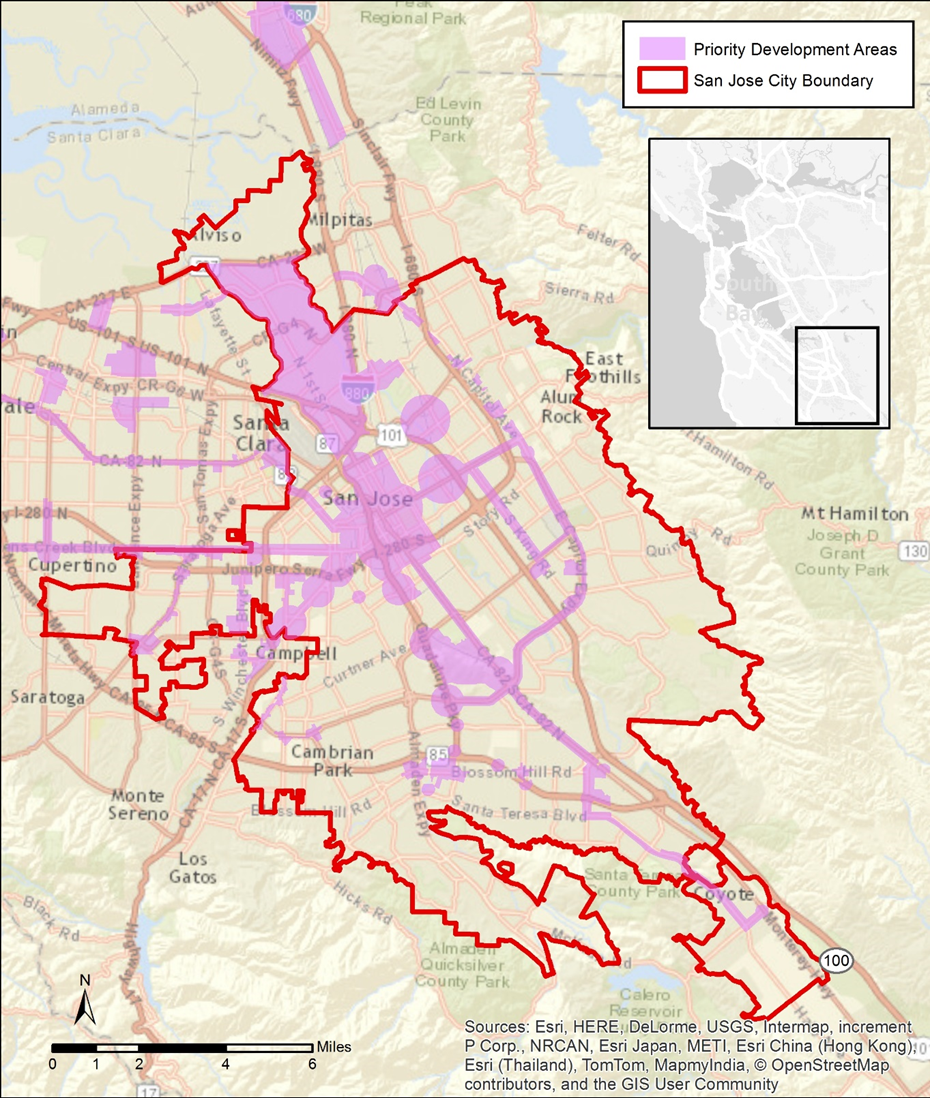
Figure 3-1 City of San Jose and Proposed Urban Villages
3.1 Case Study Objective
To plan for current and future effort to incorporate GI at the City’s landscape, the City needed a planning tool to help determine areas of opportunity and constraint for implementing GI on a wide scale and embraced the GreenPlan-IT Toolkit as a Tool that meets their needs. In discussions with SFEI, the city staff decided to use the redevelopment of the Urban Village as a case study area to test the applicability of the Toolkit. The objective of the pilot study was to demonstrate the capacities and usability of the GreenPlan-IT Toolkit in identifying feasible and cost-effective GI locations at a watershed scale. Results from the Toolkit application will be used to: 1) identify specific green infrastructure projects; 2) support the City’s current and future planning efforts, such as the development of the San Jose Storm Drain Master Plan; and 3) help comply with future Stormwater Permit requirements. At the end of the pilot study, the city staff hoped to have opportunity maps of possible GI locations, a cost-effectiveness curve for flow or pollutant reduction, and a workable Toolkit that can be used for future GI planning efforts.
The downtown area and north San Jose were identified as environmentally and fiscally beneficial locations to develop some of the Urban Villages (Figure 3-1). The majority of this proposed new development is located within the lower part of the Guadalupe River Watershed (Figure 3-2). In consultation with the city staff, the lower part of the Guadalupe watershed was selected for the development of a GreenPlan-IT Toolkit case study. Data are available in this watershed to support the full application of the Toolkit.
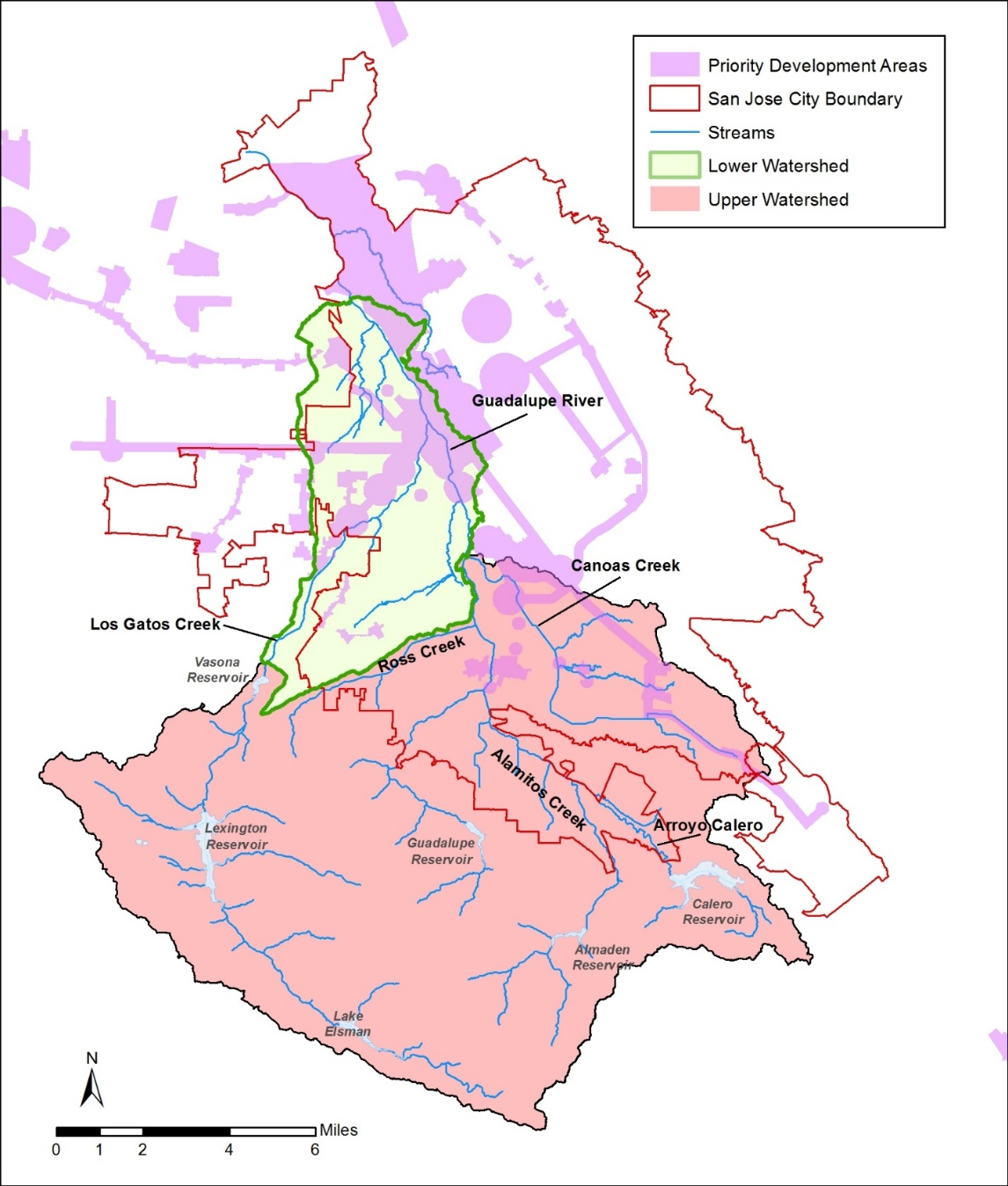
Figure 3-2 Guadalupe River Watershed and Proposed Urban Villages
3.2 Project Setting
The Guadalupe River Watershed is located in the Santa Clara Valley basin and drains to Lower South San Francisco Bay (Figure 3-2). The watershed is the fourth largest in the Bay Area with approximately 170 mi2 of total drainage area. Five main tributaries drain to the Guadalupe River. Six water conservation and storage reservoirs in the watershed provide varying amounts of flood control. The Guadalupe Watershed has a mild Mediterranean-type climate generally characterized by moist, cool wet winters and warm dry summers. Rainfall follows a seasonal pattern with a pronounced wet season that generally begins in October or November and can last to April or May, during which an average of 89% of the annual rainfall occurs (McKee et al., 2003).
The primary focus of this case study is downtown San Jose, and accordingly, the watershed boundary was adjusted to exclude upstream watersheds where gauge data are available to be included as boundary conditions for the appropriate streams and/or sub-watersheds (Figure 3-2). The resulting study area is referred herein as the Lower Guadalupe River watershed with an area of 18,613 acres.
3.3 Site Locator Tool: Data layers used and decision process
The GIS Site Locator Tool integrates regional and local GIS data and uses these data, through an identification, ranking and weighting process, to locate potential GI locations at a watershed scale. Data accuracy is an important determinant in the accuracy of map outputs produced by the Tool. The quality, scale and accuracy of the input data will determine the quality, scale and accuracy of the output maps. Therefore, it is highly beneficial to use more accurate and local data when available. When using more regional scale data layers for analyses, such as the opportunities and constraints ranking analysis, the user can weight and rank these layers to reflect the confidence in local accuracy of the data. There are many regional GIS data that are included in the Tool (Table 3-1) and additional regional data sets can be added as well. Local data sets can be added to the Tool in order to help identify potential locations that meet the goals and planning needs of each city. Each municipality will identify a set of questions or goals to answer or meet prior to running the Tool. These questions or goals become the drivers for deciding which data sets to include.
Table 3-1. Regional GIS data layers included in the Site Locator Tool.
|
GIS Data Layer Name |
GIS Data Layer Description |
|
CPAD_2014a2_Holdings |
California Protected Areas database released in the first half of 2014 |
|
FEMA_NFHL |
National Flood Hazard Layers for all BA counties |
|
Employment_Investment_areas_SCS |
From ABAG's data webpage |
|
Priority Development Areas_Current |
From ABAG's data webpage. Priority Development Areas (Current) - This feature set contains changes made to Priority Development Areas since the adoption of Plan Bay Area. DO NOT USE this feature set for mapping or analysis related to Plan Bay Area. |
|
K_12_Schools |
Schools in the bay area (point data) |
|
NLCD2011_PercentImpervious |
Percent Impervious data from the 2011 National Land Cover Dataset |
|
OSM_Buildings |
Open Street Map layer for the Bay Area _Late2014 |
|
OSM_Libraries |
Open Street Map layer for the Bay Area _Late2014 |
|
OSM_Parking |
Open Street Map layer for the Bay Area _Late2014 |
|
OSM_Parks |
Open Street Map layer for the Bay Area _Late2014 |
|
OSM_Schools |
Open Street Map layer for the Bay Area _Late2014 |
|
OSM_Streets |
Open Street Map layer for the Bay Area _Late2014 |
|
R2_CARI_PublicV |
California Aquatic Resource Inventory for Region 2 |
|
Regional_Bike_Facilities_Bay |
Regional bike facilities for the Bay Area |
|
RWQC_RB_2 |
Region 2 Water Board Boundary |
The primary drivers for GI implementation in the City of San Jose are the redevelopment Urban Villages plan and the Storm Drain Master plan. As noted previously, the Urban Villages plan focuses redevelopment in downtown San Jose for walkability, bikeability, access to public transit, and employment. The Storm Drain Master plan is a large-scale effort to analyze deficiencies in the stormwater drainage network (both storm drain and natural drainage) and provide long-term solutions to the identified deficiencies. The Plan’s goals are to improve water quality, provide flood protection, enhance and protect habitat, and increase stormwater infiltration. Together, these plans provide the pathway for future GI implementation.
San Jose also requested that infiltration trenches be added to the RBA. The Santa Clara Valley has suitable soils for infiltration to groundwater and regional large-scale infiltration trenches are being considered as one mechanism for groundwater recharge. This feature type was added and ranked for each of the five existing metrics (slope, depth to groundwater, soil type, land use, and risk of liquefaction) used for determining suitable locations.
During the first analysis for the City, potential locations were focused on parks, city-owned parcels, wide streets, existing sidewalk planters, and parking lots as potential locations for GI implementation. Formulas were developed, using existing City data, to identify streets and sidewalks with appropriate widths for implementation of bioretention features and parking lots greater than 7000 ft.². The City identified planning opportunities such as areas planned for redevelopment (PDAs), existence of stormwater infrastructure, and planned bikeways as well as constraints to GI implementation including proximity to riparian areas and gas mains. These opportunities and constraints were then categorized into factors (local development opportunities, community needs, conservation, and installation feasibility). These factors were then weighted to produce a relative ranking of areas for potential GI implementation. Community needs and local development opportunities were given the highest weight.
The City also included a data layer that identified City-owned parcels in the ownership analysis which allowed for a public/private delineation of locations in the map outputs (Table 3-2). For the Knockout Analysis, The City excluded all areas intersecting existing wetlands and proximity to other waterbodies (salt ponds, existing percolation ponds, and a 10ft buffer from creek centerlines) as well as existing GI features. The first Tool run included map outputs for bioretention units, permeable pavement, and infiltration trenches. This first run identified approximately 400 acres of moderate to highly ranked areas for potential GI implementation.
After review of the preliminary Tool outputs, city of San Jose staff decided that a second analysis, with modifications made to a few analyses, could help refine their output (Table 3-2). In particular, the City wanted to run the Tool while both including and excluding the Regional Base Analysis (two separate Tool runs). By excluding the RBA, additional locations were included in the analysis and in the map outputs. No new additions were made to the Locations Analysis while there were changes made to the Opportunities and Constraints Analysis. A data layer delineating Urban Villages was added and more heavily weighted in the local development opportunity factor. San Jose’s three-year re-pavement plan was also added and the RBA was added and ranked in lieu of running the RBA at the start of the analysis. Constraints were also removed from this analysis and layer and factor weights recalculated. Installation feasibility (existing storm drain infrastructure) was the highest weighted factor followed by local development opportunities, and community needs (planned bike paths). The City also added additional data to the Knockout Analysis including existing salt ponds and building footprints.
Table 3-2 shows the regional and local GIS data layers included in the Site Locator Tool for the City of San Mateo.
|
GIS Data Layer Name |
GIS Data Layer Description |
Data Layer Type |
Analysis |
|---|---|---|---|
|
Parks |
Layer of city parks |
Local |
Locations |
|
Sidestreet parking |
Data layer identifying streets with on-street parking |
Local |
Locations |
|
Sidewalk planter |
Data layer identifying existing sidewalk planters |
Local |
Locations |
|
Parking lot |
Data layer identifying parking lots with building footprints removed |
Regional |
Locations |
|
City-owned parcels |
Data layer identifying city owned property |
Local |
Locations |
|
Priority Development Areas |
Bay Area Wide Priority Development Areas from ABAG |
Regional |
Opportunities and Constraints |
|
Urban Villages |
Areas within the city of San Jose designated for development of urban villages |
Local |
Opportunities and Constraints |
|
Stormwater infrastructure |
Locations of stormwater mainlines buffered 80 ft |
Local |
Opportunities and Constraints |
|
Stormwater infrastructure |
Locations of stormwater manholes buffered 90 ft |
Local |
Opportunities and Constraints |
|
Stormwater infrastructure |
Locations of inlets to storm drain network buffered 60 ft |
Local |
Opportunities and Constraints |
|
Planned bikeways |
Layer showing all planned bikeways buffered 80 ft |
Local |
Opportunities and Constraints |
|
Repavement plan |
City of San Jose replacement plan buffered half of the street Face of Curb width |
Local |
Opportunities and Constraints |
|
CARI wetlands |
Wetland locations from CARI |
Regional |
Knockout |
|
Building footprint |
San Jose building footprint data layer |
Local |
Knockout |
|
Creek buffer |
Santa Clara Valley Water District 10 ft buffer for existing creeks and riparian areas |
Local |
Knockout |
|
Percolation pond |
Santa Clara Valley Water District percolation ponds data layer |
Local |
Knockout |
|
Various waterbodies |
Other waterbodies for exclusion |
Local |
Knockout |
|
Existing salt ponds |
Santa Clara Valley Water District existing salt ponds data layer |
Local |
Knockout |
|
data\SanJoseDatasets.gdb\OM_Inventory |
Data layer showing locations of existing green infrastructure |
Local |
Knockout |
|
Schools |
San Jose school data layer |
Local |
Knockout |
|
City-owned parcels |
San Jose city-owned parcels |
Local |
|
3.1 Site Locator Tool Results
During the last Tool iteration, City staff requested two Tool runs. The first run included the RBA as designed while the second run added the RBA to the Opportunities and Constraints Analysis where it was ranked and weighted. In the second run, the RBA was not included at the start of the analysis. The first run excluded many possible areas that did not meet the criteria underlying the RBA. For the second run, (including the RBA layers in a later analysis), the relative importance of these criteria can be controlled through the weighting process. City staff found the map outputs from the second analysis more helpful in the process of identifying possible GI locations as it allows for viewing all locations but provides the relative ranks for locating highest opportunity sites. Each iteration of the Tool analysis produced a map with ranked possible locations for bioretention, infiltration trench, and pervious pavement implementation (Figure 3-3). For bioretention, the final map output had a total of 9840 acres ranked from low to high potential. Eighy-five acres were highest ranked (a rank greater than 0.4), while 1705 acres were moderately ranked (a rank between .4 and .2), 3489 acres were ranked relatively low (a rank below .2), and 4559 acres were unranked.
Once the final output was produced, City staff reviewed maps through the lens of the Urban Villages planning efforts as well as other GI planning efforts. One way in which the Tool maps can be helpful is to show alternative locations when particular constraints are identified in planned locations. San Jose was exploring 5th Street and Hedding Street as a potential GI location. This location was ranked relatively lower on the map output due to the street not having an existing storm drain. City staff gave storm drain infrastructure the highest categorical weight in the analysis which resulted in the 5th and Hedding Street area being ranked relatively lower. However during review of the map outputs, a more suitable, and relatively higher ranked, location was identified nearby at 6th and Hedding.
This remote ground truthing is an important step in the process. This can also be combined with a field ground truth effort. The field effort provides real world syntax to how the Tool performed and also identifies other opportunities and constraints that the Tool didn’t capture (due to lacking data or the weighting process). City staff participated in a field ground truthing effort with the Project team. Three locations were visited: Tully Road and 7th Street, Chynoweth Avenue, and the corner of Round Table Drive and Roeder Road. The Tully Road site was identified by the Tool based on a large road median with curbed boundaries. The median is bordered by a busy three lane road, an access turn lane, and a smaller infrequently used one lane road. Discussions at the site centered on drainage patterns to existing storm drains and the potential opportunity to close the one lane road to create a larger GI feature. The Chynoweth site is already in the planning process for bioretention implementation. Site discussions centered on drainage patterns and where bulb outs could be placed. The corner of Round Table Drive and Roeder Road was selected by San Jose Staff as it was a highly ranked location that fell within an Urban Village area. This location was selected in order to demonstrate how the tool could be used to identify locations that had not previously been identified, that also met many of the City’s priorities and criteria for highly suitable locations. Outputs from the Site Locator Tool were then used in the Optimization Tool as described below.

Figure 3.3 Map output of ranked potential bioretention locations in the City of San Jose. Higher ranked locations are dark blue, lowest ranked locations are red and yellow designates unranked areas due to lacking data in those places.
3.6 Modeling Tool
The application of the Modeling Tool involved input data collection, model setup, model calibration, and finally the establishment of a baseline condition.
3.6.1 Data Collection
A large amount of data were collected to support the development of the Modeling Tool.
The input data that were used for developing a SWMM5 model of runoff for Lower Guadalupe River watershed are described below.
- Precipitation Data
The Guadalupe River Watershed is instrumented with numerous meteorological and hydrology stations (Figure 3-4). There are 11 precipitation stations operated by the Santa Clara Valley Water District (SCVWD) and the National Oceanographic and Atmospheric Administration (NOAA). There is a pan evaporation station, which is operated by SCVWD, and an evapotranspiration station, which is operated by California Irrigation Management Information Systems (CIMIS). High-resolution precipitation data (15-minute intervals) were obtained from SCVWD for 3 precipitation gauges-RF1, RF125, and RF-131, located within the Lower Guadalupe watershed (Figure 3-3). The rainfall data from 2010 to 2011 was chosen for model calibration, representing average and dry years. Annual rainfall for each precipitation station is shown in Table 3-3. The precipitation records were analyzed and compared and the Thiessen polygon method was used to assign representative weather stations to sub-basins.
- Evaporation Data
Evaporation is not as spatially or temporally variable as precipitation; hence lower resolution data from more remote sources are adequate for modeling evaporation. Monthly evaporation data for year 2010-2011 at Los Alamitos Recharge Facility in San Jose was obtained from SCVWD (Table 3-4). These data were then converted to monthly average in inches/day as required by the SWMM5 model.
- Land Use Data
The SWMM5 model requires input of land use percentages for each segment to define hydrology and pollutant loads. Land use data was were obtained from the Association of Bay Area Governments (ABAG) 2005 land GIS coverage. The coverage contains 11 different land use classifications, which were than aggregated down to six model categories. The aggregated land use groups for the SWMM5 model and their percentages are listed in Table 3-5.
- Percent of Imperviousness
The percent of imperviousness is an import input data set for SWMM5 hydrology simulation. The GIS layer of imperviousness was from National Land Cover Dataset (NLCD) 2011, which covers the entire lower 48 State at a spatial resolution of 30m pixels (http://www.mrlc.gov/nlcd2011.php). The distribution of impervious land use for Lower Guadalupe watershed is shown in Figure 3-5.
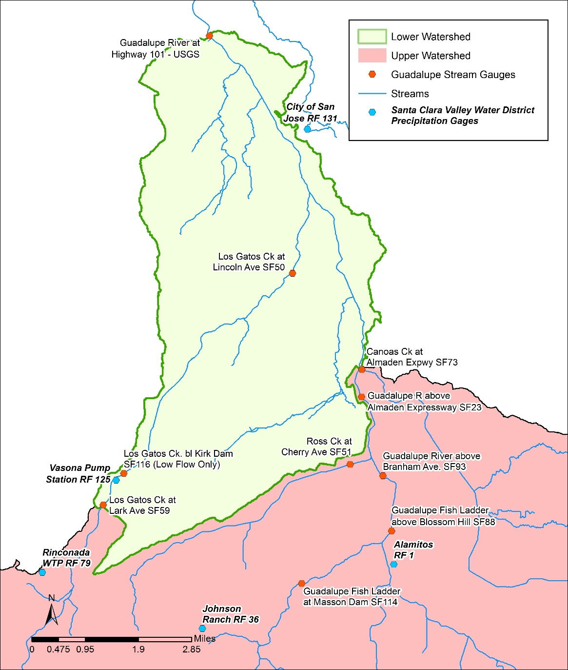
Figure 3-4 Rain gauges and Stream gages in Lower Guadalupe Watershed
Table 3-3 Annual Rainfall (inches) for Precipitation Stations
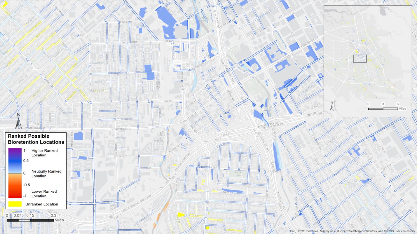
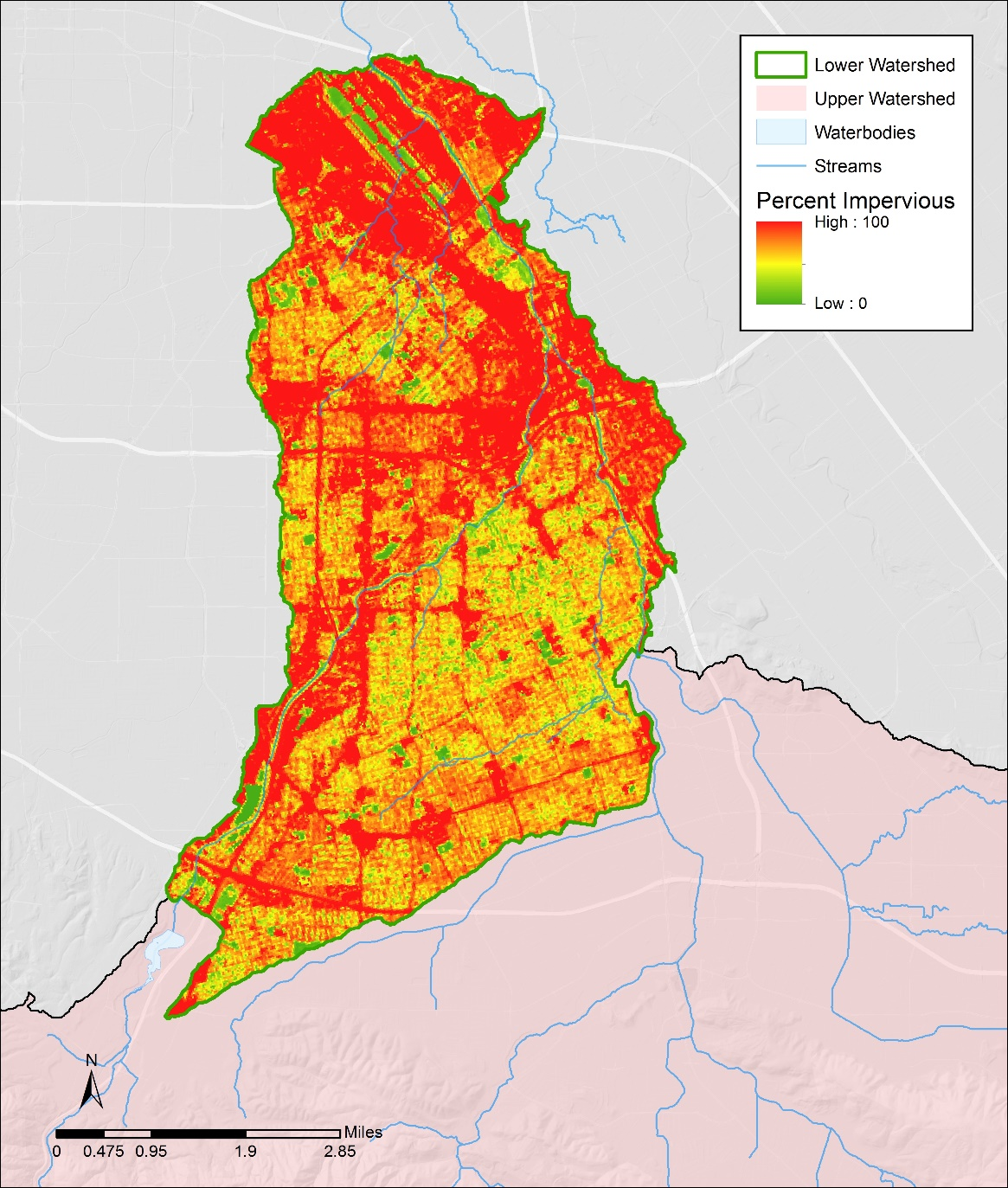
Figure 3-5 Percent of Imperviousness for Lower Guadalupe River Watershed
- Soil Data
Soil data were obtained from the State Soil Geographic Database (STATSGO) and intersected with the subbasin boundary layer to determine the percentages of each soil group for each model segment. STATSGO soils information include the hydrologic soil group (A, B, C, or D) that indicates the ability of the soil to infiltrate water. Soil type can have significant effects on the annual runoff volumes and the peak runoff rates. The Lower Guadalupe River watershed is mainly comprised of D type soils with low infiltration rates and high runoff rates (Figure 3-6).
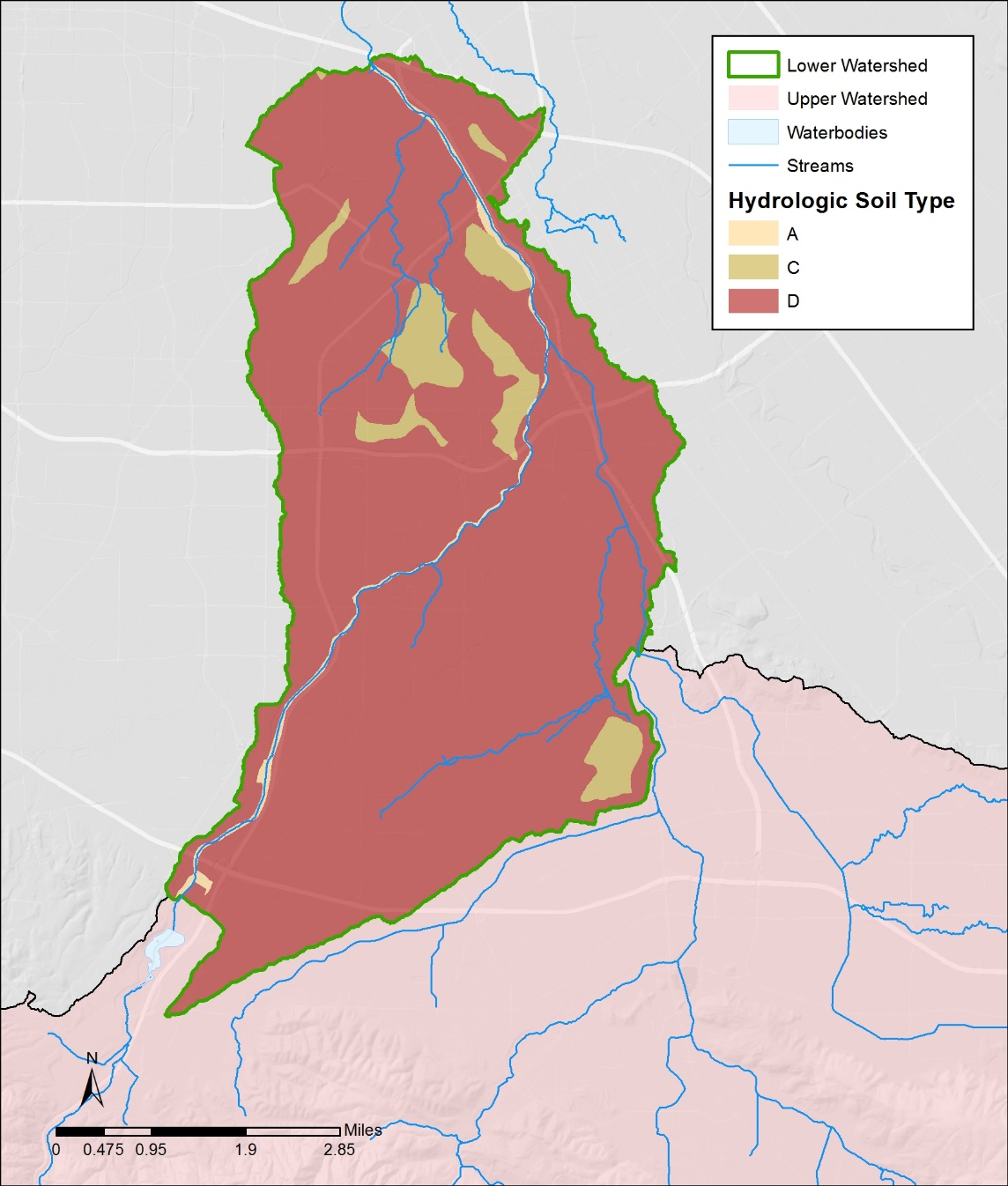
Figure 3-6 Soil Map for Lower Guadalupe River Watershed
- Inflow from Upstream
Flow data for the upstream of the Lower Guadalupe watershed were obtained from three gages at the watershed boundary. Continuous streamflow record (15 minutes interval) from 2010 -2011 was obtained from the SCVWD for stations SF23, SF73, SF59 (Figure 3-4). These data serve as the upstream boundary condition and are input into connected model segments as time series.
- Diversion Data
SCVWD operates a fairly complex water supply system in the Guadalupe River watershed that consists of storage reservoirs, ditches, percolation ponds, and pipelines. Within the modeled area, there are two gauged ditches that divert water from Los Gatos Creek. Daily flow diverted from these ditches was obtained from SCVWD for year 2010-2011. This flow was counted as loss and subtracted from inflow from station SF59.
- Calibration Data
Monitored flow data from 2010 to 2011 at two gages within the model domain were used for model calibration. Daily flow at station SF50 were provided by SCVWD. Flow from the USGS station at highway 101 were downloaded from USGS site http://ca.water.usgs.gov/data/. The USGS station receives water from the entire watershed and is the focal point of model calibration.
3.6.2 Model Setup
The first step in setting up the Modeling Tool is to delineate the watershed into smaller, sub-basins (model segments) using topographical data; the model treats each sub-basin as a homogeneous unit. Through a terrain analysis ArcGIS extension called TauDEM, the Lower Guadalupe River watershed was delineated into 150 sub-watersheds, ranging from 11 to 381 acres (Figure 3-7). Model setup also involves land use reclassification, reformatting input data into SWMM5 model formats, assigning the model segments to proper rain gauge, selecting assessment points, and estimating initial model parameters through GIS analysis and literature review. The time step of model simulation was set as 15 minutes, to be consistent with the resolution of precipitation. The model configuration established a representation of Lower Guadalupe River watershed, and model calibration was then followed to ensure the model parameters reasonably represent the watershed condition.
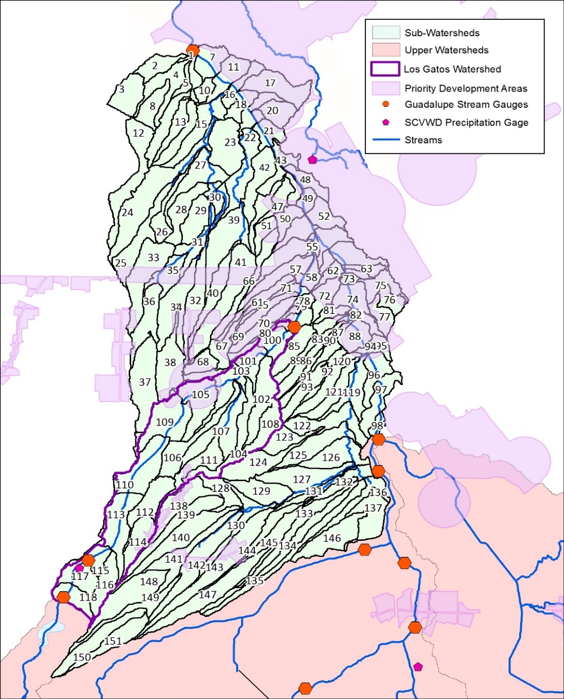
Figure 3-7 Delineated Lower Guadalupe River Watershed
3.6.3 Model Calibration
Model calibration is an iterative process of adjusting key model parameters to match model predictions with observed data for a given set of local conditions. Through the model calibration, it is hoped that the resulting model will accurately represent important aspects of the actual system. The model calibration is necessary to ensure that a representative baseline condition is established with a high degree of confidence in its applicability to form the basis for comparative assessment of various management scenarios.
The hydrologic calibration was performed at two stations (Figure 3-6) within Lower Guadalupe River watershed by means of an iterative process of trial and error using logical adjustments of parameters in consultation with local experts and technical advisors. The calibration started at the tributary station SF50 (Los Gatos at Lincoln avenue) to ensure a reasonable estimates of flow from this tributary. After the calibration was completed at this station, the calibration was then performed at the USGS station at Highway 101, near the mouth of the Guadalupe River. The calibration period was from year 2010 to 2011.
- Baseflow
SWMM5 was originally designed to simulate urban wet weather runoff but does include a method of estimating base flow (dry weather flow) (Rassman, 2010). The baseflow for the Lower Guadalupe River was determined from the measured dry weather flow in 2010 and 2011. A constant flow of 5 cfs was added to two nodes in the tributary and produced an appropriate calibration for the USGS gage.
- Calibration Parameters
SWMM5 is associated with a large number of spatially variable parameters that describe the characteristics of individual subbasins. A subset of the model parameters associated with frequent storm events - impervious percentage, subcatchment width, Manning’s roughness, depression storage, and soil infiltration parameters, are sensitive and typically used as hydrologic calibration parameters. The calibration effort was focused on adjusting these parameters until modeled flow rates match the timing, magnitude, and total volume of the observed data.
The percentage of imperviousness turned out to be the most sensitive parameter, strongly influencing both the total volume of runoff and the peak flows. To obtain a good adjustment of the hydrograph, the initial percentage of imperviousness was decreased 10% for each subcatchment. The subcatchment width is an abstract basin parameter computed by dividing the subcatchment area by the travel length. Because of its inherent uncertainty, this parameter was also used as a major tuning parameter. The travel length was increased for all basins (ranging from 50% to 100%) to create a more attenuated response to storm events. These are reasonable adjustment when taking into account the error margin that can be obtained when estimating these parameters (Wickham, et al, 2013). The parameters of depression storage, infiltration and roughness are less impactful and were adjusted within the range of the established values in the literature to help further improve model calibration.
- Hydrologic Calibration Results
The results of the final calibration are provided in Figure 3-8 and Figure 3-9. At both stations, modeled daily flow match the volume and timing of observed data well, but the peaks of biggest storms were consistently over simulated. Several factors could contribute to this. The inflow from the upstream stations makes up the majority of flow in Guadalupe River and heavily impact the calibration at downstream stations (Figure 3-5). The high flow from these stations were extrapolated from flow-stage curves that often are not calibrated or updated with field measurements during the biggest storms due to lack of personnel and sometimes hazardous conditions (SCVWD, personal communication, 2014). As a result, these flow numbers may not be very reliable and could be biased high. The model uses precipitation data from three rain gages and assigns representative stations to sub-basins based on Thiessen polygon method (Figure 3-4). Localized rainfall events, typical in the Guadalupe watershed as characterized by large variation in mean annual precipitation ranging from 48 inches in the headwaters to 14 inches at the Central San Jose, may not be captured and could contribute to the discrepancy between modeled and observed peak flows. In addition, uncertainty in some key input data such as the percent of imperviousness, local soil conditions, and directly connected impervious area could also introduce uncertainty into the model calibration.
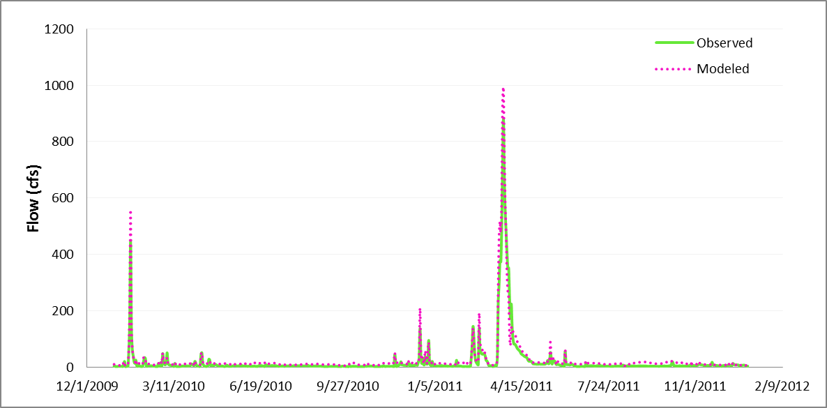
Figure 3-8. Modeled and observed daily flow at Los Gatos Creek, Lincoln Avenue
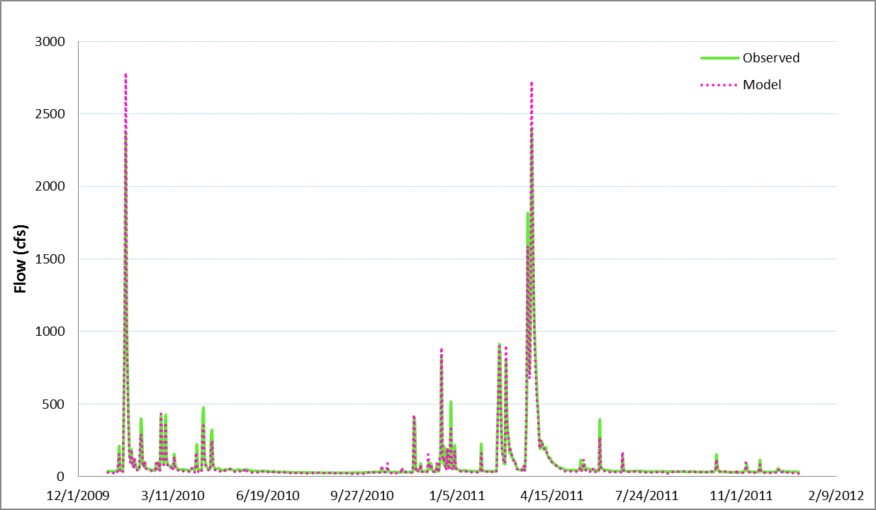
Figure 3-9. Modeled and observed daily flow at USGS station near highway 101
These caveats accepted, the accuracy of the model calibration was also quantified based on the calculated mean error for the modeled and observed storm volume and Nash–Sutcliffe model efficiency (Nash and Sutcliffe, 1970). Both statistics are well within acceptable criteria, indicating an overall good hydrologic calibration; a first indication that the model calibration is quite sufficient to support the GI application.
Table 3-6. Statistics for evaluation model calibration
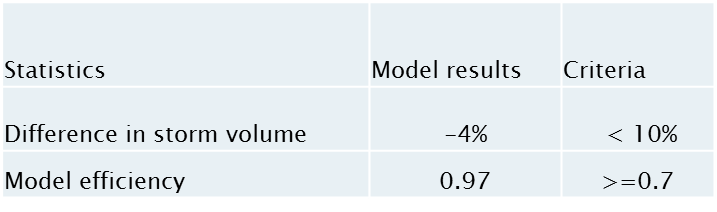
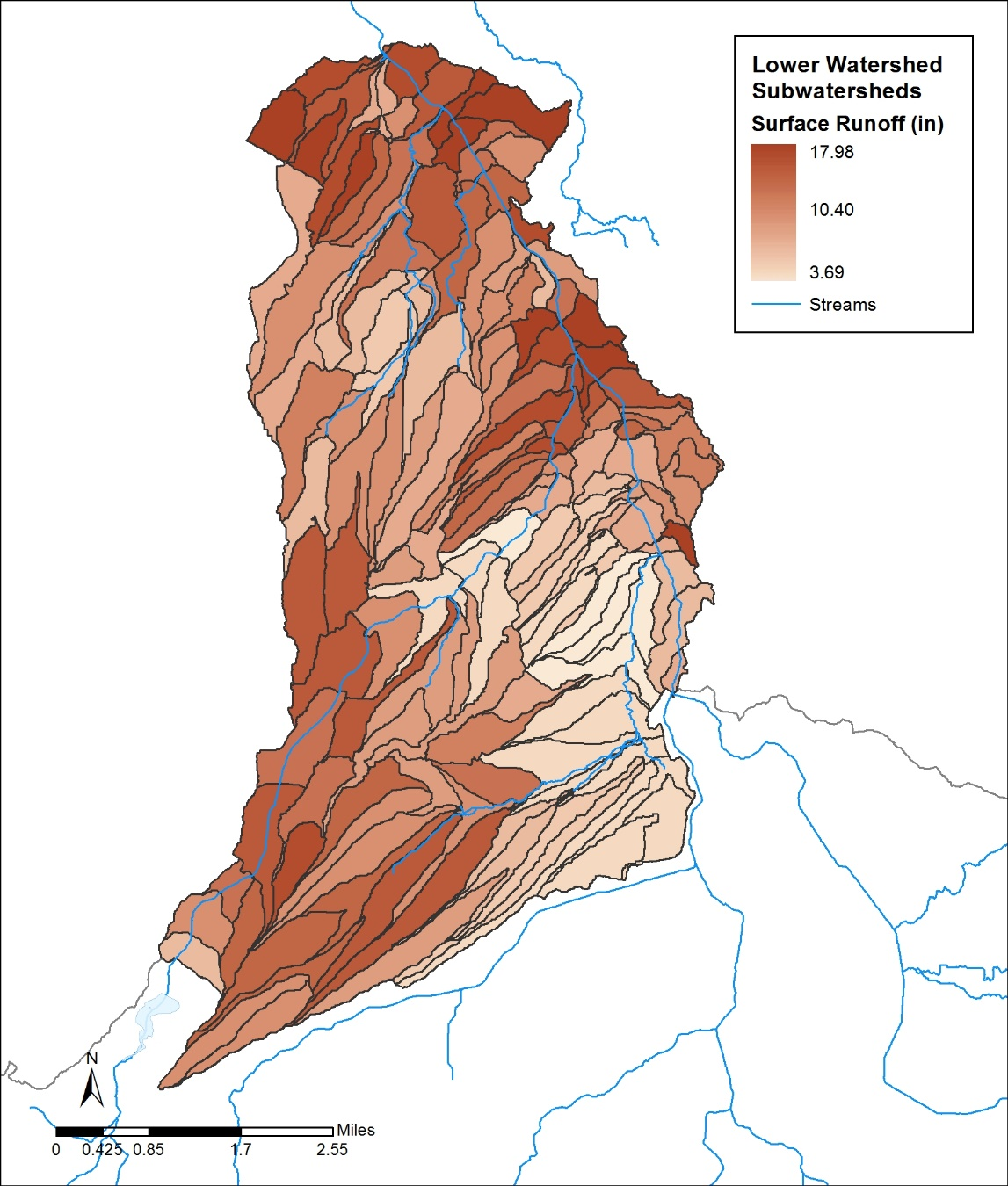
Figure 3-11. Surface Runoff Distribution for Baseline Condition
3.7 Optimization Tool
As the last tool in the Toolkit application, the Optimization Tool repeatedly runs the Modeling Tool to iteratively arrive at the optimized GI scenario. The objective of the Optimization Tool is to determine GI locations, types, and design configurations that minimize the total cost of management while satisfying water quality and quantity constraints. Currently, three GI feature types - bioretention, infiltration trench, and permeable pavement were built in the Tool, as recommended by the project Technical Advisory Committee (TAC). The major steps of this application includes formulating optimization problem, selecting critical storm, designing GI representation, and assigning GI cost.
3.7.1 Focus Area
Downtown San Jose, a primary focus area for redevelopment, was selected from the Lower Guadalupe watershed to demonstrate the application of the Optimization Tool. The selected watershed covers 53 model segments with a total area of 4300 acres (Figure 3-12). The Optimization Tool was to identify cost-effective GI combinations and distributions for the selected area, for which future GI retrofit and implementation are planned to offset the impact of the new development.
Figure 3-12. Optimization Focus Area
3.7.2 Optimization Problem Formulation
The application of the Optimization Tool began with the formulation of optimization problem, which requires the determination of management targets and selection of assessment point and decision variables.
- Management targets
The determination of management targets is the first step in formulating an optimization problem. These management targets can be based on flow and/or water quality. For example, a management target for flow can be a desired reduction in average annual volume, peak discharge, or exceedance frequency. For this case study, no specific reduction targets were defined, and the overall management targets are to reduce total runoff volume for a design storm event. Therefore, a full range of control targets from 0 -100% were explored, and the optimization was to identify optimal solutions for any possible targets within the range.
- Assessment point
An assessment point is the location in the study basin where runoff or pollutant loading reduction will be evaluated relative to optimization goals. The assessment point for this study is the outlet of the study area (Figure 3-12).
- Decision variables
To run the optimization analysis, the user must define decision variables that will be used to explore the various possible GI configurations. For this analysis, the decision variables are defined as the number of fixed-size units of the distributed GI types. In the Lower Guadalupe San Jose case study, the total number of decision variables ended up as 159 (53 basins*3 GI types). For each applicable GI type, the decision variable values range from zero to a maximum number of potential sites, which were identified by the GIS Site Locator Tool. The decision variables were also constrained by the total area that can be treated by GI within each sub-basin. Through the discussion with the project Technical Advisory Committee (TAC), a 4% “rule of thumb” (defined as GI design at four-percent of the project area to capture 100% stormwater volume of a design storm) was used to size GI for this study. During the optimization process, the combined numbers of GI were forced to be less or equal to the maximum numbers calculated by applying this 4% rule.
3.7.3 Design Storm
The setup of the Optimization Tool also required the selection of a typical precipitation year for use in comparing alternatives and assessing downstream impacts. At the recommendation of the City of San Jose, a 2-year storm with 24-hour duration was selected to drive the simulation process. The storm has a total rainfall of 1.86 inches, according to Santa Clara County’s drainage manual (Santa Clara County, 2007). The distribution of the storm was derived from a normalized rainfall pattern recommended by the manual for use in the San Jose area (Figure 3-13). To be consistent with the resolution of the storm event, the time step in the Modeling Tool as used by the optimization engine was also set at 5 minutes, different from the 15-minute time steps used in the model calibration.
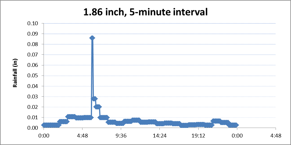
Figure 3-13. Distribution of San Jose 2-year Storm Event with 24-hour Duration
3.7.4 GI Representation
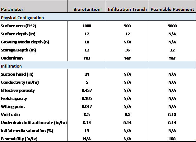
Three GI types - bioretention, infiltration trench, and permeable pavement were included for optimization. Each GI type was assigned a typical size and design configuration that remained unchanged during the optimization process. The decision variables were the number of each GI type within each sub-basin and changing in size of GIs was implicitly reflected through the change of number of GIs implemented. Table 3-5 summarizes key design parameters for each GI feature.
Table 3-6 GI configurations used in Optimization Tool
3.7.5 GI Cost
Local sources were used to derive capital cost data for GI on public rights of way. The reliable cost information for each GI feature is critical for identifying optimal solutions, because the optimization process and solutions are highly sensitive to the cost function. A unit cost approach was used to calculate the total cost associated with each GI scenario formed in the optimization process, in which cost per square feet of surface area was specified for each GI type and the total cost of any GI scenario was calculated as:
Total cost = ? (number of each LID type * unit cost * surface area of each LID type)
Implementing GI at the landscape scale would incur many costs ranging from traffic control, construction, to maintenance and operation. For this project, the costs considered were construction, design and engineering, and maintenance and operation (with 20 year lifecycle).
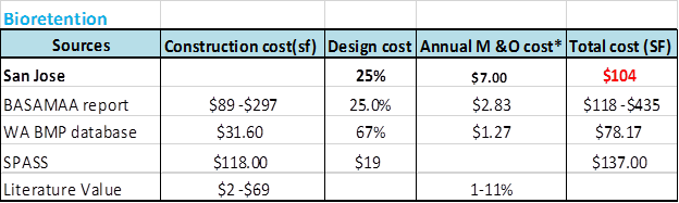
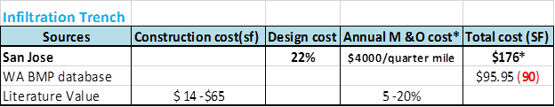
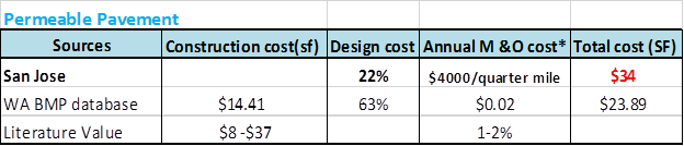
GI cost information for various GI types were collected from literature review, contacting local stormwater agencies, as well as reviewing similar studies in other regions. In general, only limited cost information was available, and these costs vary greatly from site to site due to varying characteristics, different design/configuration, and other local conditions/constrains (Table 3-7). After consulting with the TAC and stakeholders, the cost for bioretention was estimated as $104/square foot (sf) surface area, infiltration trench as $90/sf surface area, and permeable pavement $34/ sf surface area. These cost estimates were used to form the cost function in the Optimization Tool, which were evaluated through the optimization process at each iteration.
Table 3-7 GI unit costs from different sources
3.7.6 Optimization Results
Consistent with Site Locator Tool analysis, two scenarios were run with the Optimization Tool: with base analysis and without base analysis. With each scenario, the optimization procedure was run for 200 iterations, each with 100 solutions. After which, the optimization converged to final optimal solutions and the process was stopped. The entire process took about 2 hours of computer time from start to finish – a run time deemed reasonable by the TAC; a good tradeoff between spatial resolution and model usability.
- Cost-effectiveness curve
The optimization process outputs the optimal solutions along a cost-effectiveness curve. The curve relates the levels of runoff removal efficiency to various combinations of GI throughout the watershed and their associated cost. Figure 3-14 and Figure 3-15 show the cost-effectiveness curve for scenario with/without base analysis, respectively. For each scenario, all 20,000 individual solutions are plotted together, with the optimum solutions that form the left- and upper-most boundaries of the search domain highlighted in red. Each point on the graph represents one combination of the number of bioretention units, Infiltration Trench, and permeable pavement for each subarea within the study area.
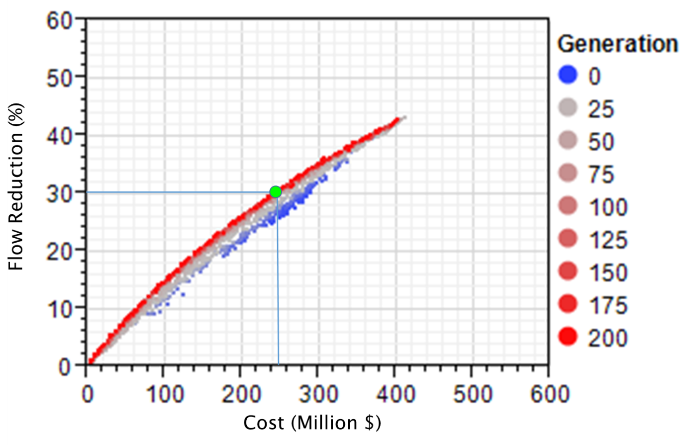
Figure 3-14. Cost-Effectiveness Curve for Scenario with Base Analysis
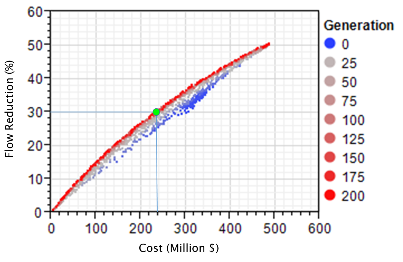
Figure 3-15. Cost-Effectiveness Curve for Scenario without Base Analysis
The cost-effectiveness curve suggests that there exists a largely linear relationship between level of implementation (represented as total cost) and runoff volume reduction, and the maximum achievable runoff volume reduction at the outlet of study area, given the objectives and constraints associated with the study, is approximately 43 percent for with base analysis (Figure 3-13) and 50 percent for without base analysis (Figure 3-14). With the help of this information, decision makers can set realistic goals on how much can be achieved and the level of investment required, as well as determine at what point further investment on GI will yield no improvement on runoff reduction. Between the two scenarios, more GIs (and thus higher cost) will be required for the with base analysis to achieve the same level of runoff reduction (i.e. 30% reduction), as the base analysis excluded some potential sites for more efficient GI types bioretention and infiltration trench, and the optimization was forced to pick more of less efficient types (incurring more cost) to make up the difference. While the cost distribution does not provide specific information about the spatial locations of actual GI features nor the actual cost of build out, knowing the types of practices associated with each point along the cost-effectiveness curve provides insight into the reasoning and order of selecting individual practices.
Of the two scenarios, the City is primarily interested in the scenario without base analysis. Therefore, the discussion of optimization results from here on was focused on this one only.
- Example scenario – 30% reduction
The optimal combinations of GI types and numbers for user-defined reduction goals along the cost-effective curve can be specified. Take the example of a 30% runoff reduction goal, the optimal combination of GI types identified through the optimization process is listed in table 3-8. In total, 3300 GIs will be needed to treat the 4300 acre focus area with a price tag of $240 million based on the model assumptions of GI design and unit cost. The number of each GI type needed for achieving certain reduction goal is generally determined by the collective factors of GI design, cost and potential feasible locations. The actual cost would be much less than the $220 M price tag given the opportunity to reduce unit costs through standardized designs batched implementation, implementation with other road related or drainage related projects, public-private partnerships, reduced need to upsize existing grey infrastructure, and many other benefits not accounted for such as increased property values, reduced heat and other benefits.
Table 3-8 The Number of GI identified for 30% Runoff Reduction

Figure 3-18 Optimal Permeable Pavement Sites for 30% Runoff Reduction
It is important to emphasize that users must interpret the optimization results in the context of specific problem formulation, assumptions, constrains, and optimization goals unique to this case study. If one or more assumptions are changed, for example, the optimization target was designed as reducing peak flow instead of total volume, the optimization might have resulted in a completely different set of solutions in terms of GI selection, distribution, and cost. It also should be noted that because of the large variation and uncertainty associated with unit GI cost information, the total cost associated with various reduction goals calculated form the unit cost do not necessarily represent the true cost of an optimum solution for the basin evaluated and are not transferable to other basins. Rather, these cost should be interpreted as a common basis to evaluate and compare the relative performance of different GI scenarios. The Optimization Tool provides a framework to identify optimal solutions for addressing stormwater management issues at the watershed level.
- Comparison with Results from Site Locator Tool
For the study area, the preliminary GIS screening through the Site Locator Tool identified 23,600 potential sites for GI implementation. These sites could serve as a starting point for GI planning and form the basis for the application of the Optimization Tool. Through the optimization process, not only were the number of sites reduced down to 3300, but the optimal combinations of GI were also identified. (Figure 3 -16). More importantly, the use of the Optimization Tool can provide users with critically needed quantification on cost and benefit (reduction) associated with various management options to help them in finding informed and optimal solutions. Therefore, the application of the full Toolkit is always preferred when sufficient data are available to support the development of the Modeling and Optimization Tools.
3.7.7 Sensitivity Analysis
Previous studies (USEPA 2011, State of Washington 2013) suggested that the optimal process and solutions are highly sensitive to GI cost. A sensitivity test was run to test sensitivity of optimal solutions to GI unit cost estimates. The unit cost for each GI type was changed (Table 3-9), and the optimization procedure was similarly run for 200 iterations with a population size of 100.
Table 3-9 GI unit cost for sensitivity analysis
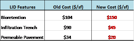
As expected, the sensitivity results suggest that assumptions made with GI cost were highly influential on the optimization modeling results. Varying the unit cost, at the same level of reduction results in different price tags and GI combinations or vice versa (Figure 3-19). For instance, at the 30% runoff reduction level, the total price tag will be $220 million with the original unit cost, but $200 million with the new cost. And the optimal combinations of GI types and numbers are also different. Therefore, reliable and accurate local cost information should be used to drive the optimization process, wherever possible.
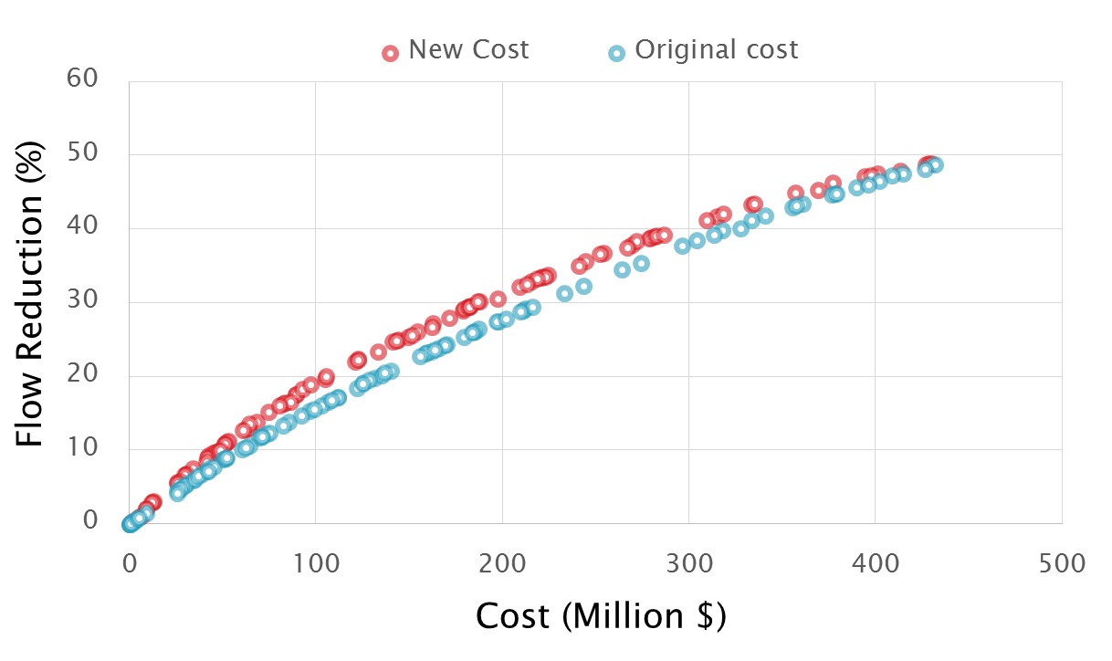
Figure 3-19. Optimal Fronts of Sensitivity Tests