![]() Optimization Tool User Manual 2020.pdf
Optimization Tool User Manual 2020.pdf
Optimization Tool User Manual
Prepared by
SAN FRANCISCO ESTUARY INSTITUTE
4911 Central Avenue, Richmond, CA 94804
Phone: 510-746-7334 (SFEI)
Fax: 510-746-7300
July 2020
Table of Contents
1. OVERVIEW
1.1 GreenPlan-IT
1.2 Optimization Tool Overview
1.3 Optimization Algorithm
1.4 Structure of Optimization Tool
2. FORMULATION OF OPTIMIZATION
3. INSTALL OPTIMIZATION TOOL
4. RUN OPTIMIZATION TOOL
4.1 Create Input Files
4.2 Run the Tool
5. REVIEW AND INTEPERATE OUTPUTS
6. FUTURE UPGRADES
7. REFERENCES
OVERVIEW
1.1 GreenPlan-IT
GreenPlan-IT is a planning tool that was developed over the past five years with strong Bay Area stakeholder consultation. GreenPlan-IT was designed to support the cost-effective selection and placement of Green Infrastructure (GI) in urban watersheds through a combination of GIS analysis, watershed modeling and optimization techniques. GreenPlan-IT comprises four distinct tools: (a) a GIS-based Site Locator Tool (SLT) that combines the physical properties of different GI types with local and regional GIS information to identify and rank potential GI locations; (b) a Modeling Tool that is built on the US Environmental Protection Agency’s SWMM5 (Rossman, 2010) to establish baseline conditions and quantify anticipated runoff and pollutant load reductions from GI sites; (c) an Optimization Tool that uses a cost-benefit analysis to identify the best combinations of GI types and number of sites within a study area for achieving flow and/or load reduction goals; and (d) a tracker tool that tracks GI implementation and reports the cumulative programmatic outcomes for regulatory compliance and other communication needs. The GreenPlan-IT package, consisting of the software, companion user manuals, and demonstration report, is available on the GreenPlan-IT web site hosted by SFEI (http://greenplanit.sfei.org/).
1.2 Optimization Tool Overview
The optimization tool of GreenPlan-IT can be used to identify and prioritize the most cost-effective GI implementation among the many options available in urban and developing areas. The tool uses an evolutionary optimization technique, Non-dominated Sorting Genetic Algorithm II (NSGA-II), to systematically evaluate the benefits (runoff and pollutant load reductions) and costs associated with various GI implementation scenarios (location, number, type, and size of GI) and identify the most cost-effective options for achieving desired flow mitigation and pollutant reduction at minimum cost. Figure 1-1 shows an example GI scenario that specifies types and numbers of GI features within different sub-basins (locations). Within GreenPlan-IT, the optimization tool is structurally designed as a standalone module to provide flexibility for the user community, but it needs interaction with other tool components to function. The optimization tool uses the site information generated from the GIS Site Locator tool as input data and interacts with the modeling tool during the search process in an iterative and evolutionary fashion to generate viable GI scenarios and compare their performance. Therefore, running the tool requires the running of both the Site Locator Tool and Modeling Tool (http://greenplanit.sfei.org/).
The optimization tool is designed to help local watershed planning agencies to develop stormwater management plans and coordinate watershed-scale investments to meet their program needs. It is intended for knowledgeable users familiar with the physics of GI and the technical aspects of watershed modeling. The tool outputs, combined with other site specific information.

1.3 Optimization Algorithm
Belonging to the family of evolutionary optimization techniques, NSGA-II is one of the most efficient and widely used multi-objective optimization algorithms that is capable of producing optimal or near-optimal solutions that describe tradeoffs among competing objectives (Deb, et al, 2002). NSGA-II incorporates a non-dominating sorting approach that makes it faster than any other multi-objective algorithm and uses a crowded comparison operator to maintain diversity along the Pareto optimal front (Srinivas and Deb, 1994). Examples of the use of NSGA-II for addressing environmental problems have been reported in the EPA SUSTAIN applications (USEPA 2009) as well as many case studies in the literature (Bekele and Nicklow, 2007; Bekele, et al, 2011; Maringanti, et al, 2008; Rodriguez, et al, 2011). The major operation steps of NSGA-II are described below.
-
Creation of First Generation
The algorithm begins with random generation of an initial population of potential solutions. The population is sorted based on the concept of Pareto dominance (non-domination) into each front. A solution is non-dominant to another solution when itperforms no worse than the other solution in all objectives, and better than the other solution in at least one objective. At the end of the sorting, each solution is assigned a fitness (or rank) equal to its non-dominant level, with a smaller rank indicating that the solution is dominated by fewer other solutions. In addition, a crowding distance, defined as the size of the largest cuboid enclosing a solution without including any other solution in the population, is calculated for each individual solution as a measure to maintain solution diversity. Large average crowding distance results in better diversity in the population.
-
Optimization Process
In the first step of the optimization process, parent populations are selected from the population by using binary tournament selection based on the rank and crowding distance. An individual solution is selected if the rank is lesser than the other solutions or if crowding distance is greater than the other solutions. The selected population generates an offspring population of the same size from the processes of crossover and mutation. The combined population of the current parent and offspring is sorted again according to non-domination and only the best N individuals are selected to form a new parent population, where N is the population size. Elitism is ensured in this step because both the parent and the child populations are used in the sorting. Comparison of the current population with previously identified non-dominated solutions are performed at each iteration. The new parent population is then used to create a new child population, and the process continues until the stopping criteria are met. At that point, the optimization is considered converged at an optimal front and the process can be stopped.
-
Stop Criteria
The users can stop the NSGA-II using some user-defined stop criteria. The commonly used criteria include maximum number of iterations; no change in the new parent population for two consecutive loops; and no tangible improvement for the fitness function after a certain number of iterations.
1.4 Structure of Optimization Tool
Structurally, the optimization tool is built around three functionalities each supported by a group of subroutines: Optimizer, GI performance evaluator, and cost calculator. The optimizer serves as the optimization engine that generates GI scenarios and drives the search process through the NSGA-II algorithm. The GI performance evaluator is used to create input files for the modeling tool to incorporate the generated GI scenarios, runs the model with new input files, and passes GI performance data generated by the model back into the optimizer. The cost calculator is used to estimate the cost of each GI scenario and to pass that information into the optimizer.
The optimization tool was written in FORTRAN language. The coding of NSGA-II was verified with example problems provided at Deb, et al (2002) to make sure the optimization algorithm was implemented correctly. The maximum number of iterations was used as stop criteria.
2. FORMULATION OF OPTIMIZATION
The formulation of the multi-objective optimization problem involves defining optimization objectives, determining decision variables, and identifying associated constraints.
-
Optimization Objectives
The optimization objectives used in this tool are to: 1) minimize the total relative cost of GI scenarios; and 2) maximize the total PCBs load reduction within a study area.
-
GI Types and Design Specifications
Four GI types - bioretention, permeable pavement, tree well (proprietary media), and flow-through planter, are currently included in the Optimization Tool, but other types could be added by an advanced user. Each GI type is assigned typical size and design configurations that were reviewed and approved by the Technical Advisory Committee (TAC) (Table 2-1). These design specifications remain unchanged during the optimization process. But if a user wants to use different design specifications for these four types, or have four totally different GI types to fit their specific needs, this can be easily achieved by changing the GI attributes in both the SWMM template file and the LID input file for optimization (discussed in Section 3).
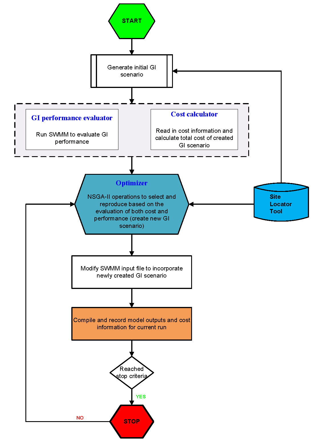
Figure 1-2. Flowchart of Optimization Tool
While current template files for the tool only include four GI types, the tool is set up to take up to six GI types. If a user is interested in other GI types, they can specify them in both the SWMM file and optimization input file, but including more than six GI types will require minor changes and recompilation of source code.
Table 2-1. GI types and configurations currently used in the Optimization Tool.
|
GI Specification |
Surface area (sf) |
Surface depth (in) |
Soil media depth (in) |
Storage depth (in) |
Infiltration rate (in/hr) |
Underdrain |
Sizing factor* |
Area treated (ac) |
|
Bioretention |
500 (25x20) |
9 |
18 |
12 |
5 |
Yes: Underdrain at drainage layer |
4% |
0.29 |
|
Permeable pavement |
5000 (100x50) |
0 |
24 |
100 |
Yes: 8 inch for underdrain |
50% |
0.23 |
|
|
Tree well |
60 (10x6) |
12 |
21 |
6 |
50 |
Yes: Underdrain at bottom |
0.4% |
0.34 |
|
Flow-through planter |
300 (60x5) |
9 |
18 |
12 |
5 |
Yes: Underdrain at bottom |
4% |
0.17 |
* In relation to the drainage management area of the unit.
-
Decision Variables
In the optimization, since GI design specifications were user specified and remained constant, the decision variables were therefore the number of units of each of the GI types in each of the subbasins within a study area. For each applicable GI type, the decision variable values range from zero to a maximum number of potential sites as specified by the boundary conditions identified by the GIS SLT.
-
Constraints on GI Locations
For each GI type, the number of possible sites is constrained by the maximum number of potential sites identified by the GIS locator tool. The decision variables were also constrained by the total area that can be treated by GI within each subbasin. Through discussion with the TAC, a sizing factor (defined as the ratio between GI surface area and its drainage area) for each GI type was specified and used to calculate the drainage area for each GI and also the total treated area for each scenario (Table 1-1). During the optimization process, the number of GI units is adjusted down when their combined treatment areas exceed the available area for treatment within each subbasin.
-
Stop Criteria Used
The maximum number of iterations is used as the stop criteria for the tool. The total number of iterative runs needed for the optimization process to converge to the optimal solutions is dependent on the number of decision variables, model simulation period, and the complexity of the model (number of sub-basins and stream network). For the current setup, 200 iterations were deemed sufficient after several test runs with different numbers. This number can be changed or different stop criteria can be used if so desired, but doing so will require modification of source codes and a thorough understanding of the optimization algorithm and consideration of computation time. Depending on the formulation of optimization problem, the optimization process could take a few hours to several weeks, and more iterations leads to longer computation time. In general, the computational efficiency can be achieved through reducing the number of decision variables, simulation time, and complexity of the problem.
3. INSTALL OPTIMIZATION TOOL
The optimization tool is designed to run under the Windows 2003/2013/NT/XP/Vista/7/10 operating system of a typical personal computer. To install the optimization tool and get ready to use it on your PC, follow the steps below:
-
Check that your Windows PC meets the system requirements.
-
Create project directory/folders to store the tool and input/output files. The main project folder can be under any root directory with any user-defined name. An example might be: “c:\My Folders\Optimization\”. Within the main folder, create three sub-folders as:
.\Binary.\Input.\Output
-
Download the tool package from GreenPlan-IT website: http://greenplanit.sfei.org/books/toolkit-downloads. Save the executable in the Binary folder and example input files in the Input folder.
-
Save SWMM5.exe in the Output folder.
4. RUN OPTIMIZATION TOOL
The optimization tool, as it currently stands, can be run as a console application from the command line within a DOS window. The steps of running the tool are as follows:
4.1 Create Input Files
Three input files are required to run the optimization tool. Each file needs to be created according to the specific format provided by the template files. All of them should be stored in the folder. \Input.
-
Basin_info.csv. This file contains total acreage and percent impervious of each sub-basin, as well as maximum number of feasible sites for each GI type within each sub-basin. The maximum number of possible GI sites are identified by the GIS Site Locator Tool and used as a constraint to the optimization.
-
LID_info.csv. This file contains three GI configuration parameters - surface area, surface width, and % of initial media saturation, and also sizing factor and unit cost for each GI type. Any of them in this file can be changed and customized to reflect local design and cost. The rest of GI configuration parameters are specified in the SWMM input file.
- SWMM_input.inp. During the optimization process, the Optimization Tool calls the Modeling Tool (SWMM5) to evaluate each GI scenario against the baseline condition. A SWMM input file needs to be created as the base for the model run, using the Windows version of SWMM5 for its easy-to use interfaces and many features. The majority of GI configuration parameters listed in Table 1-1 also need to be specified in this file (LID_CONTROLS section).
4.2 Run the Tool
Currently, the tool is set up to run in Windows command prompt:
1. Open a command prompt window;
2. Enter the path of the Optimization tool (Optim.exe), then add the path of project directory (the folder containing ‘Input’ and ’Output’ subfolders) after a SPACE.

3. Press ‘ENTER’ and run the tool.
At current setup, user only needs to specify the project folder that contains input/output folders to run the tool. Users can define their own project folder. Two caveats need to pay attention:
1. The structure of the project folder and the names of related files should follow the example below:

2. It is recommended to avoid space in the paths of the optimal tool and project folder. If there are space existing in the path, quote each path with quotation marks and then run the tool.
The key NSGA-II parameters are hardcoded, with number of generation = 200, population size =100, crossover probability=0.9 and mutation probability =0.1. The next phase of tool development will strive to make the tool more flexible to allow users to determine key NSGA-II parameters such as the number of iteration and population size.
5. REVIEW AND INTEPERATE OUTPUTS
The optimization tool produces a text file that contains reduction and cost information for all solutions and also saves SWMM input files for all intermediate solutions. All of these files are stored in the folder ./Output. The number of intermediate SWMM files can be in the order of tens of thousands, and thus, large hardware space is needed to store these files.
-
cost_reduction.txt. This is the main output file that contains generation#, population# within each generation, cost, and runoff volume reduction and percentage. Users can grab the information here to make the cost-reduction curve using Excel or other software. The reduction information in this file is needed to help you identify the optimal solution associated with specific reduction goal. For example, if a 30% reduction is desired, users can go to the file and find the generation # and population# with reduction closest to 30%. The optimal solution can then be extracted from the SWMM input file with the identified generation # and population#.
-
SWMM files for baseline. The SWMM files for baseline condition is created at the beginning of the optimization process to serve as the basis for comparison of various GI scenarios. This is done by removing any GI types in [LID_USAGE] section in the input file (.inp). The resulted report file (.rpt) after SWMM run provides baseline runoff and loads that are used as the basis to calculate their percent removal. Therefore, these files should be kept in place as removing them will crush the tool.
-
SWMM input files. The SWMM input file (.inp) for each generated GI scenario was saved to keep a record of the optimization process, and most importantly to track the optimal combinations of GI number and types. The files are named as SWMM_input_g#_p#, where g represents generation, p as population and # as the number of generation and population. For example, SWMM_iput_g002_p080.inp represents SWMM input file for generation 2 and population 80. Once users identify the targeted file, they can click open the file and mine the optimal LID solutions from the [LID_USAGE] section. For the current setup, about 40,000 files are generated that requires 10~15GB of storage.
By design, the SWMM output files are not saved in order to avoidcreating too many files that would take up a lot of computer storage space. If a user is interested in reviewing the model results from any scenarios created during optimization, one can simply run SWMM with the model input file for that particular scenario, and review model report file (.rpt) for runoff, pollutants, and GI performance information for the entire basin as well as each individual sub-basins.
It is important to emphasize that users must interpret the optimization results in the context of specific problem formulations, assumptions, constraints, and optimization goals unique to their study. If one or more assumptions are changed, the optimization might have resulted in a completely different set of solutions in terms of GI selection, distribution, and cost. It also should be noted that because of the large variation and uncertainty associated with unit GI cost information, the total cost associated with various reduction goals calculated form the unit cost do not necessarily represent the true cost of an optimum solution for the basin evaluated and are not transferable to other basins. Rather, these costs should be interpreted as a common basis to evaluate and compare the relative performance of different GI scenarios. The optimization tool provides a framework to identify optimal solutions for addressing stormwater management issues at a watershed level. Its application must be preceded by an intimate understanding of the study area and the influential factors affecting stormwater of the study area.
6. FUTURE UPGRADES
To ensure the optimization tool is comprehensive and flexible enough to handle a variety of situations/questions, the tool needs to be continuously evolving. Possible future enhancements to the optimization tool include:
- More flexibility
At current setup, the input file names/paths and many important decision variables such as the total number of iterative runs and the size of population were predetermined and hardcoded to expedite the tool development. The next phase of the tool development could make key decision variables of an optimization problem as user-defined inputs to provide flexibility for broad applicability. Also, the tool is currently tailored toward stormwater volume and pollutant load reduction, future upgrades are needed to enable the tool to handle a variety of management targets on both water quantity and quality.
- More GI types
Four GI types are included in the optimization tool at present stage that are accepted by Bay Area’s stormwater permits and recommended by municipalities and the TAC, and up to six can be customized by users. As a next step in development, more GI types as well as centralized regional facilities such as enlarged bioretention may be included in the mix to develop a diverse set of management options for a wide range of stormwater management problems.
7. REFERENCES
Bekele, E. G. and Nicklow, J. W. (2007). Multi-objective automatic calibration of SWAT using NSGA-II, Journal of Hydrology, 341, 165– 176.
Bekele, E. G., Lian, Y. and Demissie, M. (2011). Development and Application of Coupled Optimization-Watershed Models for Selection and Placement of Best Management Practices in the Mackinaw River Watershed, Illinois State Water Survey, Institute of Natural Resource Sustainability, University of Illinois at Urbana-Champaign.
Deb, K., Pratap, A., Agarwal, S., and Meyarivan, T. (2002). A fast and elitist multiobjective genetic algorithm: NSGA-II, IEEE Transactions on Evolutionary Computation, 6(2) (2002) 182-197.
Maringanti, C., Chaubey, I., Arabi, M. and Engel, B. (2008). A multi-objective optimization tool for the selection and placement of BMPs for pesticide control, Hydrol. Earth Syst. Sci. Discuss., 5, 1821–1862.
Rodriguez, H. G., Popp, J., Maringanti, C., and Chaubey, I. (2011). Selection and placement of best management practices used to reduce water quality degradation in Lincoln Lake watershed, Water Resources Research, Vol. 47, W01507, doi:10 1029/2009WR008549.
Rossman, L. A (2010). Storm Water Management Model User’s Manual, Version 5.0, U.S.
Environmental Protection Agency. Office of Research and Development. EPA/600/R-05/040.
Srinivas, N. and Deb, K. (1994). Multiobjective Optimization Using Nondominated Sorting in Genetic Algorithms. Evolutionary Computation, 2(3):221 - 248.
USEPA (2009), SUSTAIN - A Framework for Placement of Best ManagementPractices in Urban Watersheds to Protect Water Quality, EPA/600/R-09/095.
USEPA (2011), Report on Enhanced Framework (SUSTAIN) and Field Applications for Placement of BMPs in Urban Watersheds, EPA 600/R-11/144.