Description
What is Low Impact Development and why do we need it?
GreenPlan-IT Tool Overview
- Bioretention (with and without an underdrain as two different types) cells are small, vegetated, shallow depressions that serve to filter stormwater from impervious surfaces during rainfall events. Pollutants are removed from stormwater through adsorption, microbial activity, plant uptake, sedimentation, and filtration. Bioretention with out underdrains are more suitable to areas with higher soil filtration rates.
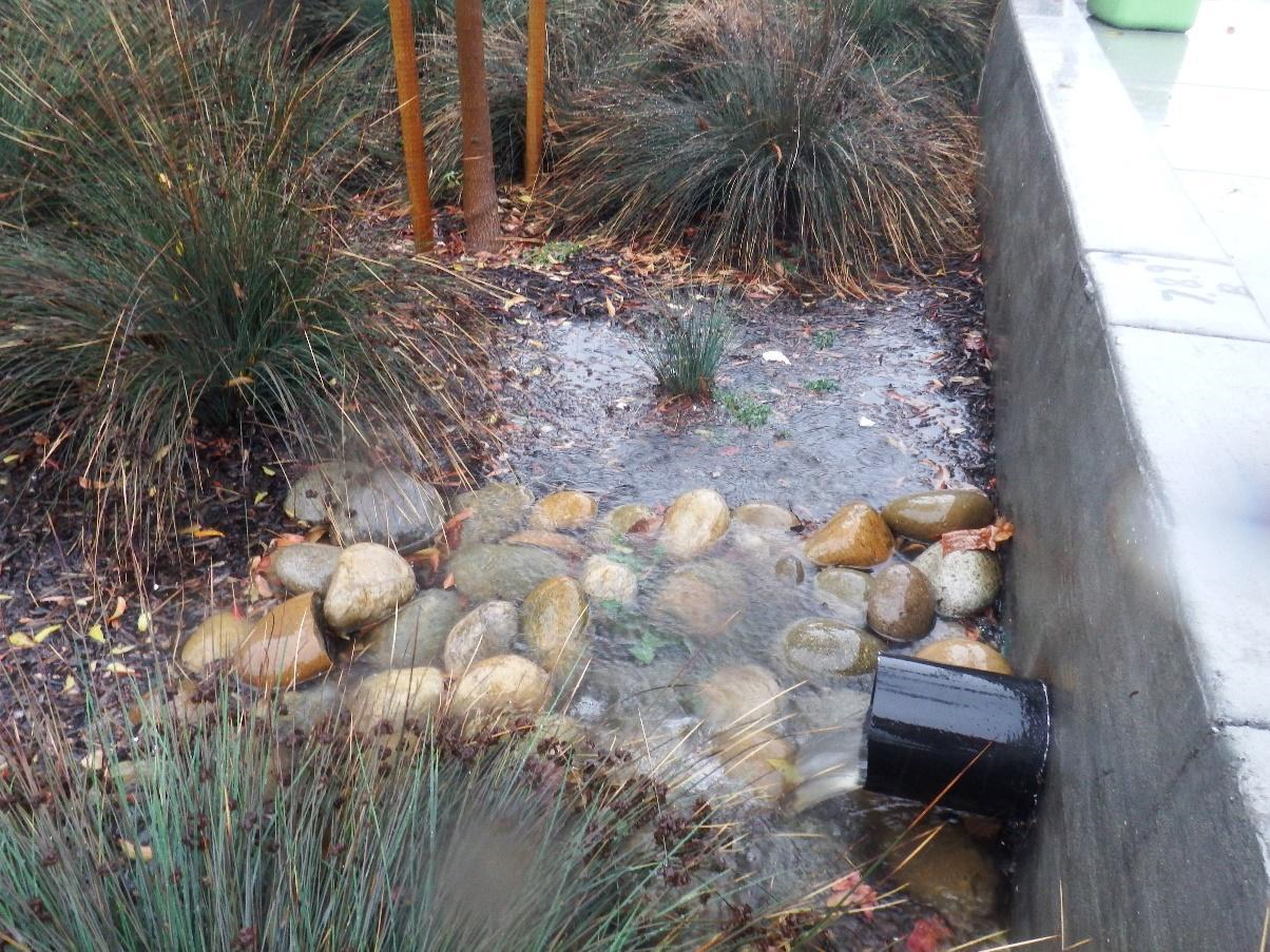
- Infiltration trenches are narrow trenches that have been back-filled with stone. Runoff is collected during storm events and stored in the void spaces of the gravel before being released back into the soil by infiltration.
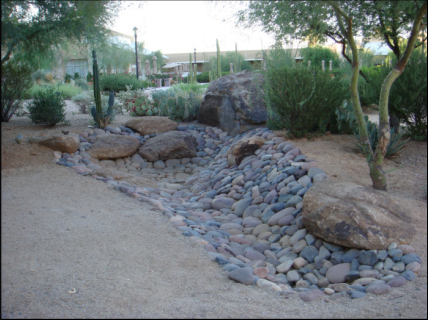
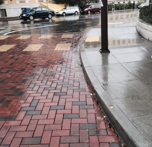
- Permeable pavement, or pervious pavement, is a porous surface laid over uniformly graded stones. It reduces runoff volume, peak discharge rates, pollutant loading, and runoff temperature.
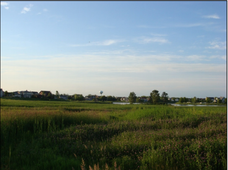
- Storm water wetlands collect runoff and store it in a permanent pool. Stormwater runoff drains into these wetlands and the plants and soils act as a filter for the stormwater.
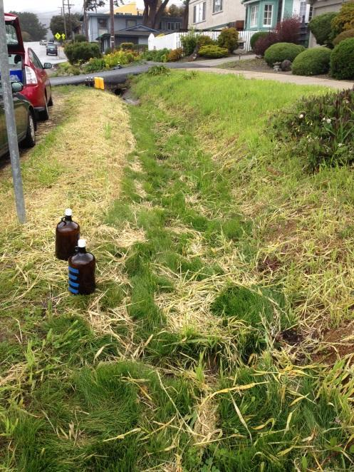
- Vegetated swales are broad, shallow channels with dense vegetation covering the sides of the slopes and bottom. They are designed to slow stormwater runoff and filter out particulate pollutants, and promote infiltration before reaching the stormwater drain.
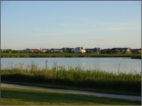
- Wet ponds are used instead of a dry detention basin to provide flood control with enhanced amenities and aesthetics and improved pollutant removal. A wet pond provides similar benefits to stormwater wetlands, except they are typically deeper and may increase the temperature of runoff.
- Flow Through Planter boxes are bioretention systems with an impermeable lining. Water stored in the planter box is disharged through a pipe not through infiltration of native soils.
Figure 7. Flow Through Planter.
- Tree Well boxes are small-scale bioinfiltration systems that are highly adaptable for small places. Tree wells are designed to collect runoff to allowing excess water to infiltrate into native soil or be collected by an underdrain.
Figure 8. Tree well example by Filtera.
Site Locator Tool User Inputs
Regional Base Analysis
- Depth to water table
- Slope
- Hydrologic soil type
- Land use
- Liquefaction risk
- Surface imperviousness
Refining Analyses
- Locations Analysis
- Ownership Analysis
- Local Opportunities and Constraints Analysis
- Knockout Analysis
Regional Datasets
See here for a description of the regional datasets provided.
Local Datasets
See Tool Preparation, I. Compiling Local Datasets.
Introduction to File Structure and Necessary File Types
- Download the SiteLocatorTool_GreenPlanIT_SFEI.zip here.
- Navigate to the SiteLocatorTool_GreenPlanIT_SFEI.zip; right-click on the zip file→Extract All…→Extract the contents to a folder.
- If you would like to store the tool elsewhere, move the extracted folder and its contents to your desired location.
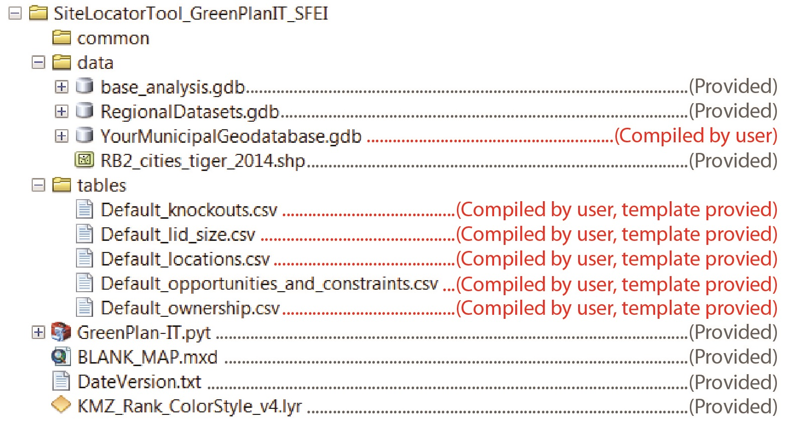
SFEI has provided the GreenPlan-IT Site Locator tool (with ancillary files), the regional base analysis, and the regional datasets in a preset folder schema, as shown below. If using local datasets, the user should reference the folder schema to determine the locations and formats of any compiled data. This will be described in detail in Tool Preparations.
Tool Preparations
Compiling Datasets
- Create a new file geodatabase for your local datasets in the “data” folder.
- We recommend renaming your file geodatabase using the convention YourMunicipalityNameDatasets.gdb (i.e. ContraCostaDatasets.gdb).
- Save/export any relevant datasets to this new file geodatabase.
- The default spatial reference used by the GreenPlan-IT Site Locator Tool is NAD 1983 California Teale Albers (EPSG: 3310). As a best practice, we recommend projecting any local datasets to this spatial reference; however, this is not a requirement.
Preparing Analysis Tables
- Open locations.csv in the “tables” folder.
- For each regional/local dataset to be included, use the locations.csv, Field Metadata to determine entries in each table field. An example of a completed locations.csv table is here: Example locations.csv.
- Save locations.csv.
- Open ownership.csv in the “tables” folder.
- For each regional/local dataset to be included, use the ownership.csv, Field Metadata to determine entries in each table field. An example of a completed locations.csv table is here: Example ownership.csv.
- Save ownership.csv.
- Open opportunities_and_constraints.csv in the “tables” folder.
- For each regional/local dataset to be included, use the opportunities_and_constraints.csv, Field Metadata to determine entries in each table field. An opportunities_and_constraints.csv table is here: Example opportunities_and_constraints.csv.
- Ranking process:
- To fill out the opportunities and constraints table, first you list all of the layers under layer name with it’s associated layer path, alias, query, and buffer size.
- Then you rank that layer as either a positive or negative factor for ranking a GI location. If it is negative, type “-1” under “rank” if positive then type “1”.
-
Next, you organize all layers into factors such as:local development considerationinstallation feasibilitycommunity needsfunding opportunitieswater quality, etc.(you can also make up your own factors and/or put all layers within one or two factors).
- Factor weight: Assign a weight to each factor such that the sum of all factor weights = 1 (for example, .25 for Local Development and .75 for installation feasibility if those were the only two factors you were using). A higher number indicates a higher weight for a particular factor. Provide this value to each layer row that the factor applies to.
- Layer weight: Within each factor, assign a weight to each layer so that the sum of the layer weights within each factor = 1. A higher number indicates a higher weight for a particular layer. If there is only one factor within that layer then the weight of that layer as 1.
- This table then runs nested weighted sums in order to produce a final ranking for each lid potential location. Note, you may choose to edit the opportunities and constraints table after viewing results. This is often an iterative process in order to create the most useful output for a user. Or you could purposely run it different ways for each neighborhood if there are specific local interests that are more or less important.
- Save ownership.csv.
- Open knockouts.csv in the “tables” folder.
- For each regional/local dataset to be included, use the knockouts.csv, Field Metadata table to determine entries in each table field. An example of a completed knockouts.csv table is here: Example knockouts.csv.
- Save knockouts.csv.
Preparing GI Size Table
- Open gi_size.csv in the “tables” folder.
- Adjust the values in the “ave_size_sqft” as desired/necessary. An example of a completed lid_size.csv table is here: Example gi_size.csv. See gi_size.csv, Field Metadata for field descriptions.
- Save gi_size.csv.
Loading the GreenPlan-IT Toolbox
- Open a new map document in ArcMap.
- If the ArcToolbox Window is not open, click the ArcToolbox button
 on the Standard Toolbar.
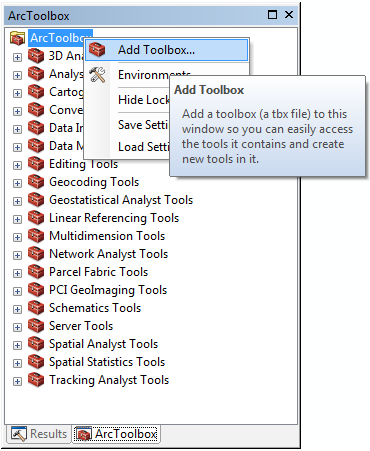
 - If the GreenPlan-IT Tool is not visible in the ArcToolbox Window…
- Right-click ArcToolbox.
- Select Add Toolbox…
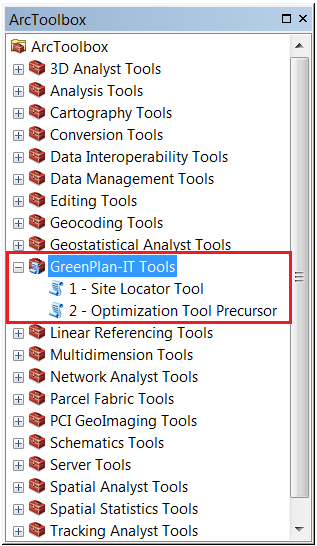
- Browse to the location of the SiteLocatorTool_GreenPlanIT_SFEI folder, and select the GreenPlan-IT.pyt toolbox file.
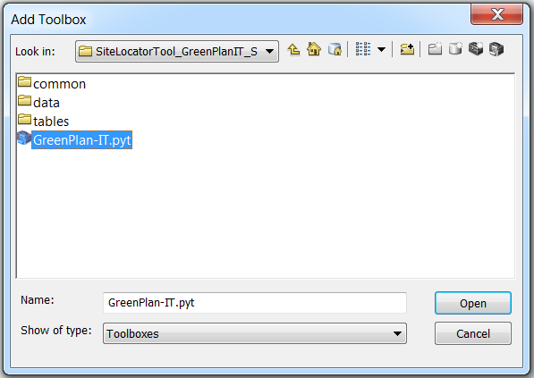
- Click Open.
- The GreenPlan-IT Toolbox has now been added to the ArcToolbox Window.
1 - Site Locator Tool
- 8 GB RAM (required); 16 GB RAM (recommended)
- 64-bit background geoprocessing
- Spatial Analyst Extension
- Double-click 1 – Site Locator Tool in the GreenPlan-IT Toolbox.
- The tool will open to the following interface:
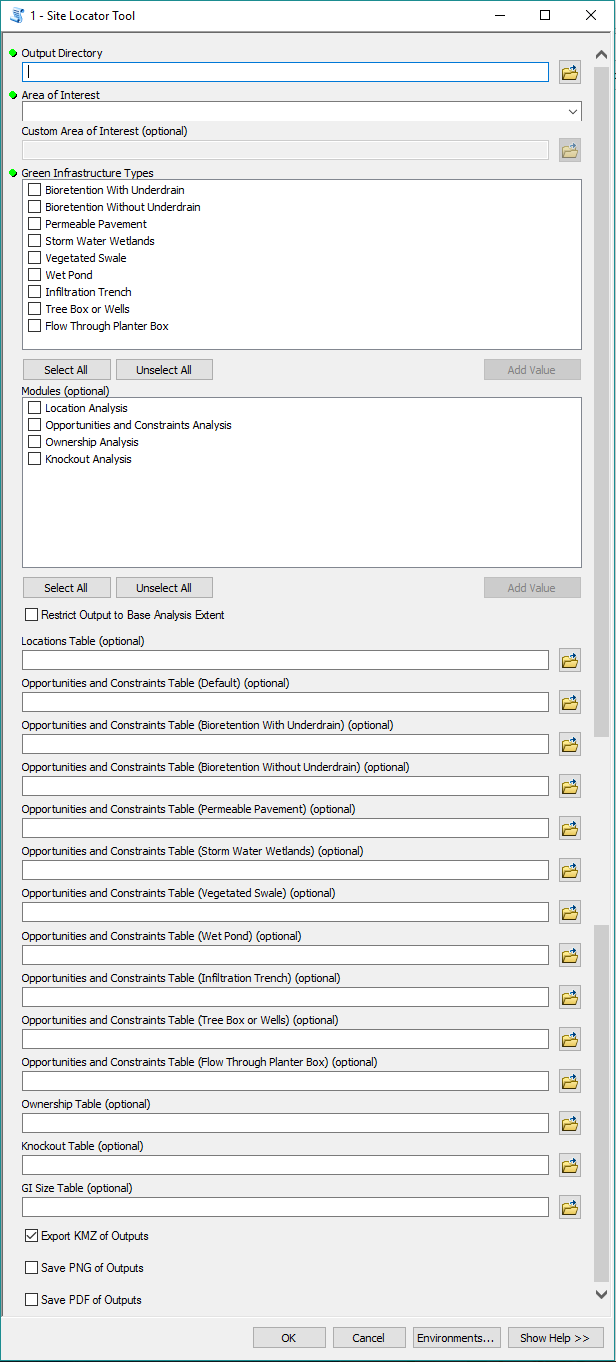
- Output Directory: Select the folder where you would like the site locator tool outputs to save. We recommend that the character length of the output directory be < 100 characters.
- Set the extent: You may set the extent by (a) selecting an Area of Interest or (b) setting a Custom Area of Interest using a polygon feature class with a single feature containing the desired boundary area.
- To select an Area of Interest: Use the Area of Interest dropdown menu and select the desired area.
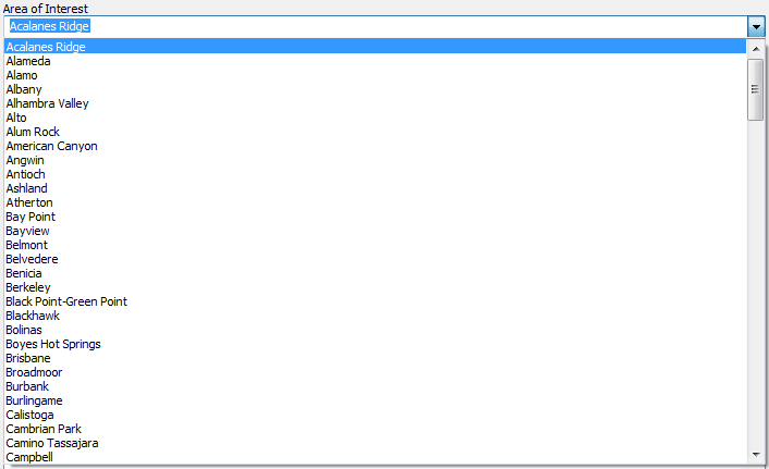
- To select a Custom Area of Interest: Select "[Custom Area of Interest]" under the "Area of Interest" field. This activates the "Custom Area of Interest (optional)" field which you can then specify the polygon feature class containing your custom boundary.
- To select an Area of Interest: Use the Area of Interest dropdown menu and select the desired area.
- GI Types: Select at least one GI type to include in the Site Locator analysis.
- Modules (optional): Select the modules/additional analyses to be included when running the tool.
- Restrict Output to Base Analysis Extent: SFEI has provided a base analysis for each of the nine (9) GI types. Check to restrict the final outputs to only areas that overlap the regional suitability layer for each GI type.
- Note: The base analysis layers can be incorporated two ways: (1) Check “Restrict Output to Base Analysis Extent”to exclude all locations that are NOT identified as suitable area for each GI type in the base analysis. (2) Do not check “Restrict Output to Base Analysis Extent” to prevent results from being limited to locations identified as suitable for each GI type in the base analysis. You may still include the base analysis layer in the Opportunities and Constraints module and run the tool for that type of GI only, in order to rank locations that fall within the base analysis areas as higher. This second option may be the preferable method. See Preparing Analysis Tables.
- Module Tables (optional): Table paths should only be provided for selected modules/analyses.
- Locations Table: If you selected the Location Analysis module, navigate to and select your locations.csv table.
- Opportunities and Constraints Table (Default and GI specific): If you selected the Opportunities and Constraints Analysis module, navigate to and select your opportunities_and_constraints.csv table for each GI type.
- Note: you can specify a "Default" Opportunities and Constraints Table which will be used for any GI types that do not have a GI specific Opportunities and Constraints Table specified.
- Ownership Table: If you selected the Ownership Analysis module, navigate to and select your ownership.csv table.
- Knockout Table: If you selected the Knockout Analysis module, navigate to and select your knockouts.csv table.
- GI Size Table: If using average GI sizes in the Site Locator analysis, navigate to and select your gi_size.csv table.
- Export KMZ of Outputs: Check to generate KMZs of the GI locations; these may be viewed in Google Earth or Google Maps.
- Note: The KMZs generated by the GreenPlan-IT Site Locator Tool contain simplified feature polygons and should be used for general viewing purposes only. Any analysis should be performed using the feature classes in the file geodatabase.
- Save PNG of Outputs: Check to export a PNG map of the outputs. The legend provided with the tool will have to be added manually.
- Save PDF of Outputs: Check to export a PDF map of the outputs. The legend provided with the tool will have to be added manually.
- Click OK to run. (The tool may take several hours to run to completion, depending on the size of the area of interest, the number of GI types selected, and the number of modules included.)
Understanding the Outputs
Final File Geodatabase of Outputs
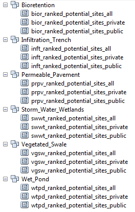
- A ranking will only be applied when the Opportunities and Constraints Analysis has been applied.
- Feature classes ending in “_private” or “_public” separate GI locations into the private and public domains, respectively. These feature classes are only generated if a distinction between private/public areas has been made in the Location Table and/or Ownership Table.
GI Location Feature Class Description
GI Area by Rank
KMZ Exports
Messages and Summaries
2 – Optimization Precursor Tool
Running the Tool
- Double-click 2 – Optimization Precursor Tool in the GreenPlan-IT Tools toolbox.
- The tool will open to the following interface:
- Input Geodatabase: Select the file geodatabase generated from the Site Locator Tool. The name of this geodatabase will have a name similar to LID_Site_Suitability_AreaOfInterest_yyyy.mm.dd_hh.mm.ss.gdb.
- Output Directory: Select the folder where you would like the Optimization Precursor Tool outputs to save.
- Sub-basin Feature Class: Select a polygon feature class containing the sub-basin boundaries for the area of interest.
- Sub-basin ID: Use the dropdown menu to select a unique ID field from the Sub-basin Feature Class. If a unique ID field does not exist, use the Object ID field.
- GI Types: Select the GI types to include in the Site Locator analy.
- GI Size Table: Navigate to and select your lid_size.csv table.
- GI Size Table Unit: Select the unit of measure in the GI size table: (SQUARE) FEET or (SQUARE) METERS.
- Ownership Domains: Use the dropdown menu to select the ownership domain.

- Click OK to run.
Understanding the Outputs

